The Heckscher-Ohlin (H-O Model) is a general equilibrium mathematical model of international trade, developed by Ell Heckscher and Bertil Ohlin at the Stockholm School of Economics.
It builds on David Ricardo’s theory of comparative advantage by predicting patterns of commerce and production based on the factor endowments of a trading region.
The Ricardian model of comparative advantage has trade ultimately motivated by differences in labour productivity using different technologies. Heckscher and Ohlin did not require production technology to vary between countries, so the H-O model has identical production technology everywhere.
Ricardo considered a single factor of production (labour) and would not have been able to produce comparative advantage without technological differences between countries. The H-O model removed technological variations but introduced variable capital endowments recreating endogenously the inter-country variation of labour productivity that Ricardo had imposed exogenously.
ADVERTISEMENTS:
Bertil Ohlin famous book, Interregional and International Trade was published in 1933. Although he wrote the book alone, Heckscher is credited as co-developer of the model, because of his earlier work on the problem and because many of the ideas in the final model came from Ohlin’s doctoral thesis supervised by Heckscher.
The model essentially states that international trade occurs because countries differ in their relative factor endowments and commodities differ in their relative factor intensities. Relative endowments of factors of production (land, labour and capital) determine a country’s comparative advantage. Countries have comparative advantages in those goods for which the required factors of production are relatively abundant and cheap locally. This is because the prices of goods are ultimately determined by the prices of their inputs. Goods that require inputs that are locally abundant will be cheaper to produce than those goods than require inputs that are locally scarce.
On the basis of relative factor endowments, countries may be categorized as capital abundant or labour abundant or land abundant countries. Similarly on the basis of relative factor intensities, goods may be grouped as capital intensive or labour intensive or land intensive goods. For example, a country where capital is abundant but labour is scarce will have comparative advantage in the production of capital intensive goods that require lots of capital but little labour. If capital is abundant, its price will be low.
As it is main factor used in the production of capital intensive goods, the price of these goods will also be low and thus attractive for both local consumption and export. Labour intensive goods, on the other hand, will be very expensive to produce since labour is scarce and its price is high. Therefore, the country will be better off importing those goods.
ADVERTISEMENTS:
Thus, in its full development the H.O. theorem lends powerful support to traditional doctrine. It provides a full-fledged explanation of why production costs might differ from one country to another and it shows the possible causes of relative commodity cheapness.
Definition of Relative Factor Abundance:
(i) Physical Definition:
A country is called capital-abundant provided the ratio of quantity of capital to quantity of labour in that country is greater than the corresponding factor quantity ratio in the other country irrespective of the fact whether or not the ratio of price of capital to price of labour in that country is less than the corresponding factor price ratio in the other country.
ADVERTISEMENTS:
For example, country I is said to be capital abundant relative to country II, if country I is endowed with more units of capital per unit of labour relative to II, that is, if the following inequality holds :
qC1/qL1 > qC11/qL11
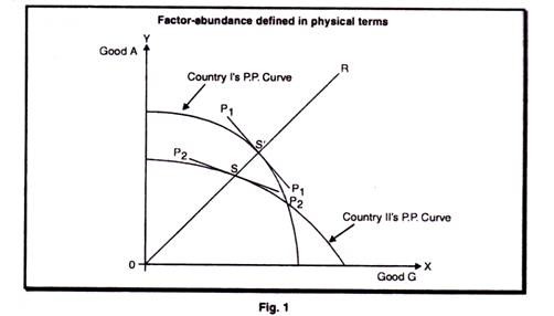
Where C1 is the total amount of capital in country I, L1 is the total amount of labour in country I, and C11 and L11 are the total amount of capital and labour, respectively in country II. We will now show that if country 1 is abundant in capital according to this definition, it implies that country 1 has a bias in favour of producing the capital intensive good. The nature of this bias is best illustrated by figure 1. It is assumed in the figure that good A is capital intensive good and good B is labour intensive good. If both countries were to produce the goods in the same proportion, say along the ray OR country 1 would be producing at point S’ on its production possibility curve and country II would be producing at point’s on its production possibility curve. The slope of country is production possibility curve at S’ is steeper than the slope of country ll’s curve at S.
This implies that good A would be cheaper in country I than in country II, and that good B would be cheaper in country II than in country I, were the two countries producing at the respective points. This is also illustrated by the fact that the commodity price line P1P1 is steeper than the line P2P2. The opportunity cost of expanding production of good A is, therefore, lower in country I than in country II, and vice versa for good B. This shows that country 1, the capital rich country, has a bias in favour of the capital intensive good from the production side, and that the country abundant in labour, country II, has a bias in favour of producing the labour intensive good.
It does not follow from this, however, that the labour rich country will export the labour intensive good. It might be the case that demands factors more than offset the bias from the production side. Such a case is illustrated in figure 2, which contains the same production possibility curves as in figure 1, and good A is still the capital intensive good and good B the labour intensive good. The difference is that now we have taken demand into account. Demand in the two countries is characterized by two sets of indifference curves, where the curves Io1 Io1 I11 I11 etc. represent demand in country I and curves Io11 Io11 I111 I111 etc. represent demand in country II. Demand in country I is obviously biased toward the capital intensive good and demand in country II is biased toward the labour intensive good.
Thus, in isolation good A is relatively more expensive in country I than in country II. This is shown by the fact that commodity price line P2P2 in country II is steeper than the line P1P1 representing relative commodity prices in country I.
From this it follows that when trade is opened up between the two countries, country I will export B and country II will export good A. In other words the country abundant in capital will export the labour intensive good, and the country abundant in labour will export the capital intensive good.
Leaving aside Lancaster’s definition, factor abundance can be defined in two ways in the H.O. model. The two alternative definitions physical and price are not equivalent. Only according to price definition, it follows that the country abundant in capital will export the capital intensive good and that the country rich in labour will export the labour intensive good. Thus, the H.O model directly follows when we define factor abundance in terms of factor prices and it may follow or may not follow when we define factor abundance in terms of factor proportions.
ADVERTISEMENTS:
(ii) Price Definition:
A country is called capital abundant provided the ratio of price of capital to price of labour in that country is less than the corresponding factor price ratio in the other country irrespective of the fact whether or not the ratio of quantity of capital to quantity of labour in that country is greater than the corresponding factor quantity ratio in the other country.
Country I is said to be capital abundant relative to country II if at the pre-trade autarkic equilibrium state capital is relatively cheaper in I than In II. More precisely, I is said to be capital abundant relative to II, if at the pre-trade autarkic equilibrium state, the following inequality holds:
ADVERTISEMENTS:
PC1/PL1 < PC11/PL11
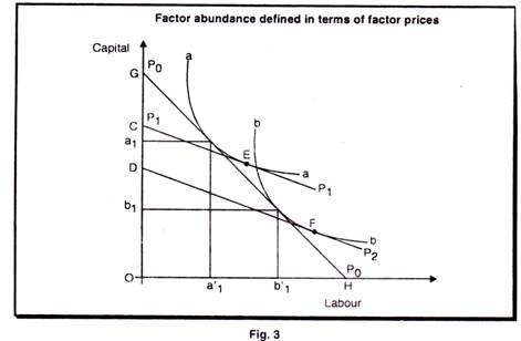
where PC1 is the price of capital in country I, PL1 is the price of labour in country I, and PC11 and PL11 are the prices in country II of I capital and labour, respectively. In other words, if capital is relatively cheap in country I, the country is abundant in capital, and if labour is relatively cheap in country II, country II is rich in labour. Country I will export the capital intensive good and country II will export the labour exclusive good. This is explained in the figure 3.
We start with two isoquants, aa and bb, which characterize the production functions and are the same in both countries. According to these isoquants, B is the labour intensive good and A is the capital intensive good. Relative factor prices in country I, where capital is cheap, are given by the line POPO. Let us assume that the isoquants represents 1 units of the respective good. Then 1 unit of good A will be produced with oa1 of labour . But capital and labour can be exchanged for each other in a ratio shown by the factor price line P0P0.therfore, oa11 of labour is worth a1G of capital and oa1of capital is worth a11H of labour.
ADVERTISEMENTS:
We said that 1 unit of good A would be produced with oa1 of capital and oa11of labour. But now we can view the line GH as a budget line or a cost line, and we can express the cost of producing 1 unit of A in terms of capital alone or labour alone. Doing so, we find that the cost of producing 1 unit of A is OG measured in capital or OH measured in labour. By applying exactly the same kind of reasoning, we also find that the cost of producing 1 unit of good B in country I is the same as that for producing 1 unit of A; that is, it is OG measured in capital and OH measured in labour.
Let us find out the cost of producing 1 unit of each good in country II. The only information we have about country II is that capital is relatively more expensive there than in country I. This means that the slope of the line representing the ratio of factor prices in country II will be less steep than the slope of PoPo.
A possible factor price line in country II is P1 P1. It is tangent to the aa isoquant at E. A parallel factor price line is P2P2– which is tangent to the bb isolquant at F. It is obvious that P2P2 must lie below P1 P1. From this it follows that the cost of producing 1 unit of good A in country II is OC measured in capital, whereas it is OD measured in capital for 1 unit of B. Thus, in country II it is more expensive to produce a given amount of good A than it is to produce the same amount of B.
If we now compare production costs in the two countries, we find that it is relatively cheap to produce good A in country I and relatively cheap to produce good B in country II. From this it follows that country I will export good A and country II will export good B. This establishes the Heckscher-Ohlin theorem that the country abundant in capital will export the capital intensive good and the country abundant in labour will export the labour intensive good.
Are the two definitions of factor abundance, namely, the physical and price definitions are equivalent? In other words, is it necessarily true that, in the autarkic pre-trade equilibrium state, capital is relatively cheaper in that country which is endowed with relatively more units of capital? Unfortunately, the answer turns out to be negative. The price definition implies relative economic abundance while the physical definition reflects merely relatively physical abundance. What is the difference between economic versus physical abundance? The former is based on the factor quantities relative to demand.
The later is based on the absolute quantities of factors that exist in each country. Factor prices on the basis of which factor abundance is decided when the price definition is used are like commodity prices, determined by both demand and supply. While the price definition is based on both supply and demand influences, the physical definition is based solely on supply ignoring completely the influence of demand.
ADVERTISEMENTS:
Hence, we cannot rule out the possibility that demand conditions might outweigh supply conditions with the result that the two definitions of factor abundance might give rise to contradictory classifications of the countries involved. For instance, assume that country I is capital abundant relative to country II on the basis of physical definition. Further assume that country I’s consumers have a stronger bias toward consuming capital intensive commodities than country ll’s consumers. Under these circumstances, it is not impossible for capital to be relatively more expensive in country I before trade. Then, country I would be classified as capital abundant according to physical definition but labour abundant according to price definition.
For completeness, it should be mentioned that a third definition of factor abundance has been proposed by Lancaster (1957) as follows:
(iii) Lancaster’s definition:
A country is said to be abundant in that factor which is used intensively by the country’s exported commodity. Is Lancaster’s definition of factor abundance appropriate for the HO. theorem? Not at all. On the basis of this definition, the HO. model is by necessity tautologically true. The H.O. model asserts that a country exports that commodity which uses relatively more intensively its abundant factor, while Lancaster’s definition calls abundant that factor which is being used more intensively by the exported commodity. On the basis of Lancaster’s definition, the H.O. theorem is by definition true and it can never be refuted. But tautologies cannot help us explain the observed structure of trade. In this connection, one Is reminded of Samuelson’s observation that “the tropics grow tropical fruits because of the relative abundance there of tropical conditions.”
The H.O. theorem is correct only when the price definition of factor abundance is used. On the basis of physical definition, H.O. theorem would predict no trade but the outcome would obviously depend on tastes. The H.O. theorem is always true on the basis of the price definition of factor abundance and in the absence of factor intensity reversals. Difficulties arise only when the physical definition of factor abundance is being used. Thus, the Heckcher-Ohlin theorem is necessarily true on the basis of the price definition of factor ambulance. But the theorem is not necessarily true on the basis of the physical definition of factor abundance.
Following the H.O. theorem we can rank goods according to factor Intensities. Let us assume country I to be abundant in capital and country II to be abundant in labour. If we rank all goods in country I according to capital intensity used in production, then, this country will first export the most capital intensive good and then go to the second most capital intensive, and so on. Similarly, country II will export its most labour intensive first, then go on to the second most labour intensive, and so on. The ranking of goods according to factor intensities is a ranking according to comparative advantage.
ADVERTISEMENTS:
As we have discussed above, according to the Heckscher-Ohlin theorem, what determines trade is differences in factor endowments.
The theorem is based on the following assumptions:
(i) There are no transport costs or other impediments to trade;
(ii) There is perfect competition is both commodity and factor markets;
(iii) All production functions are homogeneous of the first degree;
(iv) The production functions are such that the two commodities show different factor intensities;
ADVERTISEMENTS:
(v) The production functions differ between commodities, but are the same in both countries, that is good (A) is produced with the same technique is both countries and good (B) is produced with the same technique in both countries.
These are the assumptions used in connection with the Heckscher- Ohlin theorem of trade. They are necessary to state the meaning of comparative advantage in the two-by-two-by two models, and to prove the factor price equalization theorem.
Factor Price Equalization Theorem:
Trade occurs in a world where the movement of goods and the mobility of factors are more or less imperfect. It is common to assume perfect mobility of factors nationally, completely free movement of goods within and across national boundaries and complete immobility of factors internationally. Under the assumption of full mobility of factors internationally, factor prices would be the same in all countries. But in a world where factors of production cannot move between countries, whereas goods can move freely trade in goods can be viewed as a substitution for factor mobility.
Commodity trade will equalize factor prices completely only in the absence of factor intensity reversals between the factor endowment ratios of the two countries and provided that neither country specializes completely in the production of one commodity. Incomplete specialization in both countries is consistent with widely differing factor prices between countries. The factor price equalization theorem is an important corollary of the H.O. theorem.
The Assumptions of the Theorem:
ADVERTISEMENTS:
There are two countries (I and II). Each endowed with two homogenous factors of production called capital (C) and labour (L) and producing two commodities A and B.
In addition, assume the following:
(i) There is perfect competition in both production and factor markets.
(ii) There are no transport costs and other impediments to trade.
(iii) All production functions are homogeneous of the first degree (i.e., constant returns to scale).
(iv)The production functions are such that the two commodities show different factor intensities.
(v) The production function for a given commodity is the same in all countries but the production functions of different commodities are different even in the same country.
(vi) Incomplete specialization in production in each country.
The Box diagram with the same Production Functions in the two countries:
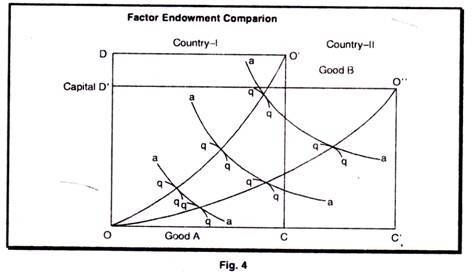
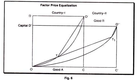
The box OCO’D represents total factor endowments in country I,
And the box OC1O11D1represents total factor endowments in country II. From this we can know that country I is abundant in capital, measured in physical amounts as C1/L1 > C11/L11 and country II is abundant in labour, using the same measure.
We measure production of good A from the lower left hand corner and production of good B from the upper right hand corner. As production functions are the same in both countries the aa isoquants are identical for both countries. The bb isoquants are also the same, in the sense that they both illustate the same production functions. Labour is measured on the horizontal axis of the box and capital on the vertical axis. From the ways the isoquants are drawn, it follows that good A is the labour intensive good and good B is capital intensive one.
Factor Prices under Autarky:
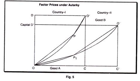
Before trade, the two countries can produce anywhere on the contract curve in their respective boxes. Let us assume that country I produces at the point P on its contract curve and country II produces at point P’. What will then be the implication for factor prices? From the figure 5, we can see that country I uses more capital intensive methods of production then country II in both lines of production. Production functions are the same in both countries and they are homogeneous of the first degree.
We know that the marginal productivities are determined exclusively by the factor intensities used in production. Because country I uses more capital per unit of labour than country II, the marginal productivity of capital at P in country I will be lower than marginal productivity of capital at P’ in country II. Factor prices are determined by marginal productivities. Prom this it follows that the price of capital will be lower in country I than in country II and that the return for labour; i.e. the wages will be higher in country I than in country II. This holds when each country produces and consumes in Isolation.
Commodity and Factor Prices under Trade: Factor Price Equalization:
Following the H.O. theorem country I, where capital is relatively cheap, will export the capital intensive good and country II will export the labour intensive good. Good B is the capital intensive good and good A is the labour Intensive one. Hence, when trade starts, country I will move along its contract curve from point P toward the O corner and country II will move from point P1 along its contract curve toward the O11 corner. Possible equilibrium points when the two countries trade are shown in figure 6. The boxes and contract curves are, of course, the same. The difference is that country I now produces at point T and country II produces at point T1. These are obviously production patterns which are possible under trade. What are the implications for factor prices?
Because of the assumption about constant return to scale marginal productivity of labour and capital will be constant along any ray from the orgin, such as OT T1. Let us de4not the marginal
productivity of labour and capital in country I in industry A and in industry B with, respectively, MPLlA, MPClA MPClB and MFCIB.
Analogously, denote the marginal productivities in the respective industries in the second country with MPLIIA, MPCIIA, MPLIIB and MPFIIB
We can see that labour and capital are used in the same proportion in industry A in both countries at T and T1. From this it follows that MPL IA MPLIIA and that MPCIA = MPCIIA. Furthermore, the line O1T is parallel to the line O11T. Hence the factors of production are combined in the same proportions in both countries in industry B, too. From this it follows that MPLIB = MPL,IIB and that MPCIIB = MPIIB.
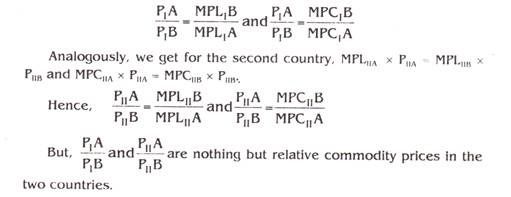
One of our assumptions is that factor markets are perfectly competitive and that factors of production are fully mobile in the country. This means that the payment for labour, the wage, must be the same in both industries and that the payment for 1 unit of capital also must be the same in both industries. The factor reward equals the marginal productivity of the factor multiplied by the price of the good produced. From this it follows the MPLIA x PIA = MPLIB x PIB and that MPCIA X PIA = MPCLIB X PIB. This gives
Under trade, they must be the same, and hence PIA /PIB = PIIA /PIIB already known that at point T and TI MPLII+A = MPLIIA MPCIA = MPCIIA, MPLIB = MPL II,B, and MPCIA = MPCII B. This gives us MPLIIA x PIA = MPLIIA X PIIA = MPLIIB X P1B = MPLIIB x PIIB x PIIB. In other words, factor prices will be completely equalized in the two countries.
The demonstration shows that as long as we can find trading points such as T and T1 as in figure-6 the implication is that factor prices will be the same in both countries. Given our present assumptions, this means that as long as both countries are incompletely specialized, that is, as long as both countries produce both goods trade will lead to complete factor price equalization.
Let us now examine the commonsense explanation of factor price equalization. Before trade, capital is cheap in country I and labour is cheap in country II. Therefore, country I has a comparative advantage in the capital intensive good (B) and country II has a comparative advantage in the labour intensive good (A).
When the two countries participate in trade, country I will export good B and country II will export good A. To increase its production of good B, country I has to move its factors of production from industry A to industry B. To produce more of good B, the producers in country I need, more capital. Therefore, the price of capital is bid up, and the relative price of what was the cheap factor before trade rises.
Similarly, the producers in country II start to produce more of good A, in order to export it. This is the labour intensive good. As more of it is produced, more labour is needed and the relative price of labour goes up. Hence trade leads to an increase, in both countries in the price of the abundant factor, the relatively cheap factor until factor, prices are the same in both countries.
Now the question is, are we always able to find trade points such as T and T’ as in figure 6. Not necessarily. The alternative is that one of the countries or possibly both, might be completely specialized and produce only one good. The more the factor endowments in two countries differ, the larger is the probability that one country will be completely specialized and that complete factor price equalization will not occur.
Complete or Partial Factor Price Equalization:
There are differences of opinion among trade theorists to the question whether commodity movement will equalize the factor prices completely or partially. Classical trade theory always took it for granted that free mobility of factors of production between different regions would tend to equalize the relative and absolute prices of productive services in the different regions. Thus, migration of labour from crowded Europe to less crowded America would result in a drop in the America’s wage rates relative to America’s land rents and relative to commodities; at the same time European land rents would fall and European real wages would rise. Migration of labour would cease only when absolute and relative factor prices had been finally equalized.
An important addition to this classical doctrine of factor price equalization has been supplied by Bertil Ohlin. In his Interregional and International Trade (1933) Ohlin has developed the highly interesting result that
(i) Free mobility of goods in international trade can serve as a partial substitute for factor mobility and
(ii) Will lead to a partial equalization of relative (and absolute) factor prices. At one point Ohlin even goes so far as to say, “it is not worthwhile to analyze in detail why full equalization does not occur; for when the costs of transport and other impediments to trade have been introduced into the reasoning, such as equalization is in any case obviously impossible.” Actually in more than half a dozen places, primarily in chapter II, OhIin definitely asserts the impossibility or improbability of complete factor price equalization, usually as if the proposition were so obvious as to require little explanation.
In 1919 Eli Heckscher stated that ‘trade will equalize factor rewards completely provided the factors of production are combined in fixed proportions. He says factor price equalization is an ‘inescapable consequence of trade”.
Something important has been added to the classical exposition by P.T. Ellsworth in his excellent work International Economics (1938). But why should there be only a tendency towards factor price equalization? Why should the equalization be only partial and incomplete? Why should free commodity movements be only partial substitute for free factor movements? This the crucial question now at issue. Ellsworth has more clearly addressed himself to this issue than OhIin, and his discussion is worth reproducing at some length: one might conclude that complete equalization of the price of the various productive factors would result (from free commodity trade).
This however, is highly improbable if not impossible. It could only occur if the demand for various kinds of labour could be concentrated largely on those areas where each kind was most abundant, thereby raising wages there to a parity with wages in scarce labour areas. Likewise, the demand for land would have to be concentrated on abundant land areas and the demand for capital on districts well supplied with capital.
Such a wholesale localization of demand, is however, quite impossible. Owing to the technical requirements of production which in the case of practically all commodities calls, not for labour, land or capital alone, but for combinations of all three of these major groups of factors. Thus, the industrial demand is always the “joint demand” for several factors.
Complete equalization of factor prices would require an unattainably perfect adaptation of demand to the highly varying local supplies of the different agents.
Moreover, did any such price equalization occur, it would contain the seed of its own destruction. For when all factor prices were everywhere the same, there would no longer be any reason for trade and with the cessation of trade, and there with the extinction of the demands which brought about the price equalization, the original disparities in factor equipment would immediately reassert themselves. It is clear that Ellsworth does believe that factor price equalization involves a logical contradiction and is therefore impossible.
It is sufficient to note that there does not appear to be in the literature a satisfactory demonstration of the necessarily partial or incomplete character of factor price equalization.
In attempting to devise a rigorous proof of the partial character of factor price equalization, Samuelson (1948) made a surprising discovery: the proposition is false. It is not true that factor price equalization is impossible. It is not true that factor price equalization is highly improbable. On the contrary, not only is factor price equalization possible and probable, but in a wide variety of circumstances is inevitable.
Specifically:
(i) So long as there is partial specialization, with each county producing something of both goods, factor prices will be equalized, absolutely and relatively, by free international trade;
(ii) Unless initial factor endowments are too unequal, commodity mobility will always be perfect substitute for factor mobility.
(iii) Regardless of initial factor endowment even if factors were mobile they would, at worst, have to migrate only up to a certain degree, after which commodity mobility would be sufficient for full price equalization.
(iv) To the extent that commodity movements are effective substitutes for factor movements, world productivity is, in a certain sense, optimal; but at the same time, the imputed real returns of labour in one country and of land in the other will necessarily be lower, not only relatively but also absolutely, than under autarky.
All of the above propositions are essentially valid whatever the number of commodities, regions and factors of production, but the empirical probability or improbability of price equalization would be altered in a complex manner by such complications.
We have discussed that given certain assumptions trade will equalize factor prices. But these assumptions can hardly be expected to be fulfilled.
