Keynesian Macroeconomic System: IS and LM Curve (With Diagram)

Introduction:

Equilibrium level of national income is determined by aggregate demand which is composed of consumption and investment expenditures (assuming a pri­vate sector economy without any trade).

Keynesian system involves six functional re­lations, viz., consumption function (or the sav­ing function), the investment function, the demand function for money, aggregate pro­duction function, the demand function for la­bour and supply function of labour.

Keynes’ saving function, money demand function and labour supply function are really different from that of the classical system. The primary determinant of Keynes’ saving function is in­come rather than the classical rate of interest. That is,

S = f(Y) … (3.24)

Keynes added the speculative demand for money, L(r), to the classical transaction de­mand for money, kPY. Thus, Keynes’ money demand function is written as

M = kPY + L(r) … (3.25)

where speculative demand for money de­pends on the rate of interest, r.

Keynes’ labour supply function is assumed to depend on money wages which are institu­tionally rigid in the downward direction. Thus, labour supply function is

S_L = f(W) … (3.26)

where W is the money wage.

However, the aggregate production func­tion, investment function, and labour demand function of Keynes do not differ from the clas­sical forms.

Keynesian income determination theory can explain macroeconomic problems once we incorporate money market in our analysis. It is the rate of interest, determined by the de­mand for money and the supply of money, that integrates goods market and money market. Rate of interest not only influences invest­ment but also (speculative) demand for money.

Thus, a synthesis of income and mon­etary analysis is brought about by the interest rate. Equilibrium national income is deter­mined in the goods market when saving equals investment. Monetary equilibrium is attained in the money market when demand for and supply of money are equal to each other.

By establishing equilibrium in the goods market and money market, equilibrium level of national income and the rate of interest are simultaneously determined. To establish the ‘general equilibrium’, we use the Hicks- Hansen tool—most popularly known as the IS-LM tool. The IS-LM analysis, a neo- Keynesian analysis, explains Keynesian mac­roeconomic system that takes into account goods market and money market, simultane­ously.

Goods Market Equilibrium: The IS Curve:

Keynesian theory of aggregate demand is inadequate to explain macroeconomic system when the money market is introduced. So, we need to establish a link between the money market and the goods market through the rate of interest. Now, we treat interest rate as a variable whose equilibrium value is deter­mined simultaneously with that of the level of income.

In the goods market, we have:

(i) the saving function,

(ii) the investment function, and

(iii) an equilibrium condition.

These are expressed as:

S = f(Y) … (3.24)

I = f(r) … (3.14)

and S = I … (3.27)

To develop the IS curve our task is to find combinations of interest rate, r, and the level of income, Y, that equate investment with saving. We cannot solve equation (3.27) for Y to determine equilibrium Y, un­less we know ‘r’. If ‘r’ is unknown, we can­not find out the volume of investment ex­penditure. At a given ‘r’, one can determine the volume of investment expenditure.

Once we determine investment expenditure, we are able to find out the equality between in­vestment and saving. Consequently, equi­librium national income is determined in the goods market. In fact, there are a series of combinations of r and Y that ensure equal­ity between saving and investment. Once these combinations are plotted on the r – Y plane, we get a curve which Hicks-Hansen called the IS curve.

The IS curve shows al­ternative combinations of national income (Y) and the rate of interest (r) which equili­brate the commodity market. Mathemati­cally, the IS curve is simply the solution of equation (3.27) for r in terms of Y.

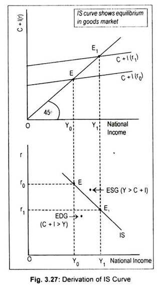
Fig. 3.27 illustrates the construction of the IS curve. In the upper panel of the figure, we have drawn the aggregate expenditure (C + I) schedule. National income is determined at that point where the aggregate demand line cuts the 45° line. We start with the given rate of interest. Suppose, the initial rate of interest is r₀. At this rate of interest, aggregate demand schedule, C + I(r₀), cuts the 45° line at E. The corresponding level of income is Y₀. As investment is inversely related to the interest rate, decrease in the interest rate from r₀ to r₁ causes investment to rise. Consequently, aggregate demand line shifts up to C + I(r₁).

The new aggregate expenditure schedule cuts the 45° line at E₁ and the corresponding level of national income rises to Y₁. Thus, for the interest rate r₀, a point of product market equilibrium will be Y₀. This r₀ – Y₀ combination is one point on the IS curve, shown in the lower panel of Fig. 3.27.

Similarly, r₁ interest rate produces Y₁ equilibrium income. So, r₁ – Y₁ combination is another point on the IS curve. By joining these points (E and E₁ in the lower panel) we get a curve known as the IS curve.

Thus, the IS curve is the locus of all equilibrium combinations of r and Y that bring product market in equilibrium. Any point off the IS curve shows disequilibrium in the goods market. To the right of the IS curve, there emerges excess supply of goods (ESG) when aggregate output exceeds aggregate demand, i.e., Y > C + I. To the left of the IS curve there arises excess demand for goods (EDG) when aggregate demand exceeds aggregate output, i.e., C + I > Y.

The IS curve slopes downwards to the right. Or it has a negative slope. Its slope depends on the saving function and investment function. The IS curve will be relatively steep (flat) if investment is less (more) sensitive to interest rate changes. The IS curve will be vertical if investment is absolutely interest-inelastic. An autonomous increase in investment expenditure or government expenditure will shift the IS curve to the right.

Alternative Method of Deriving IS Curve:

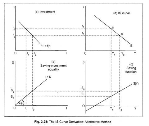
The derivation of IS curve can be made in terms of a four-part diagram (Fig. 3.28). In part (a), we have drawn investment function that shows the inverse relationship between investment and the rate of interest. Part (c) plots the saving function that represents direct relationship between income and saving. Part (b) is simply a 45° identity line, and part (d) plots the IS curve.

Suppose, the rate of interest is r₀. At this rate of interest, investment must be I₀ and, thus, the volume of saving must be S₀ necessary for equilibrium. This volume of saving implies an equilibrium income of Y₀ necessary for equilibrium. This establishes one point on part (d), say point M. If the rate of interest rises to r₁, investment declines to I₁. This results in a decline in national income to Y₁. With this level of income the volume of saving becomes S₁ (< S₀). This establishes another point on part (d), say point N.

The procedure may be repeated for each level of income (interest) to obtain corresponding values of interest rate (income value) that ensures equality between saving and investment. By joining all these equilibrium points, we get an IS curve drawn in part (d).

Thus, the IS curve shows various combina­tions of income and interest rate that brings commodity market in equilibrium.

The IS curve is negatively sloped. Its slope depends on the nature of saving and investment functions.

The IS curve may shift if there is a change in autonomous consumption, private investment and government expenditure and taxes.

Autonomous increase in consumption demand, private investment expenditure and government spending cause IS schedule to shift to the rightward direction while an autonomous increase in taxes causes a leftward shift of the IS schedule. However, an equal increase in both taxes and government spending leads to a rightward shift of the IS curve.

Properties of IS Curve: Summary:

(i) The IS curve is the equilibrium combinations of income and interest rate such that the product market or goods market is in equilibrium.

(ii) The IS curve slopes downward to the right because an increase in interest rate causes investment expenditure to decline, therefore, reduces aggregate demand and, hence, equilibrium national income.

(iii) Its slope depends on the saving and investment functions. The IS curve will be relatively steep (flat) if investment is less (more) sensitive to interest rate changes.

(iv) This IS curve will shift by an autonomous change in investment spending or government spending.

(v) Any point on the IS curve shows that there is neither excess supply nor excess demand for goods. Any point off the IS curve shows either excess supply of goods (ESG) or excess demand for goods (EDG).

A Mathematical Example on the IS Curve:

First, consider a two-sector economy. Assume the following equations for investment and saving.

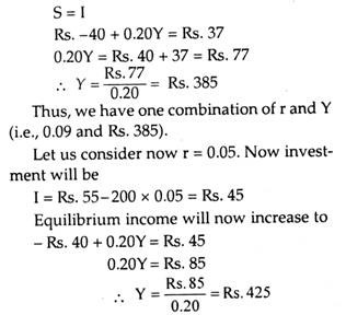
I = Rs. 55-200r and S = – Rs. 40 + 0.20Y.

With these equations, we derive an IS schedule for a two-sector economy, given the interest rate r = 0.09 p.c.

Solution: Given the interest rate r = 0.09 p.c. investment, I = Rs, 55 – 200 x 0.09 = 55 – 18 = Rs. 37. Equilibrium requires

Thus, another combination of r, and Y (i.e., 0.05 and Rs. 425) is obtained.

By plotting these r-Y combinations, we obtain negatively sloped IS curve.

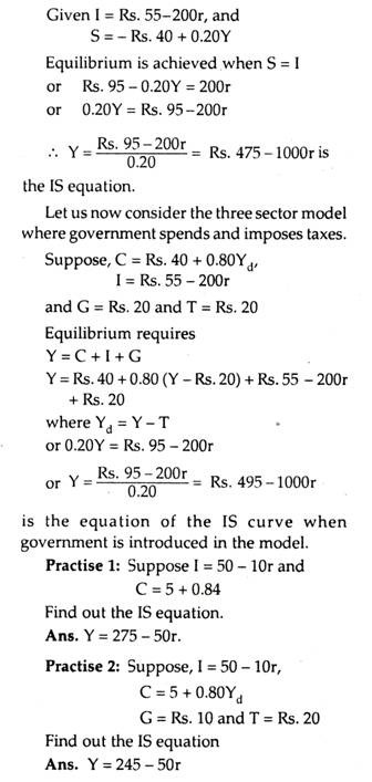
Now, we will derive the equation for IS with the help of the following equations:

III. Money Market Equilibrium: The LM Curve:

Equilibrium in the money market occurs at that point where money demand equals money supply. In the Keynesian system, money demand for transaction purposes
depends on the level of income and money demand for speculative purposes depends on the rate of interest.

Thus, the money demand function, denoted by M_d, can be expressed as:

M_d = f(Y, r) … (3.28)

Supply of money (M) is institutionally given. Given M , corresponding to each level of income there is a rate of interest which produces equilibrium in the money market. Money market equilibrium occurs when

M = M_d … (3.29)

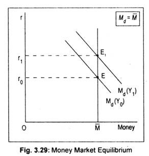
The LM curve shows different combina­tions of r and Y that equilibrate money market. In Fig. 3.29 we have drawn two money demand schedules, corresponding to two different levels of income. At Y₀ income, money demand schedule is given by M_d (Y₀). As income increases from Y₀ to Y₁, the money, demand curve shifts to the right. The vertical line M shows fixed money supply.

We find equilibrium in the money market when money demand schedule intersects money supply schedule. We start with a given income, Y₀. At Y₀ level of income, money demand schedule is M_d (Y₀). The rate of interest is r₀. As income rises to Y₁, money demand schedule shifts to M_d(Y₁) and the rate of interest rises to r₁. Thus, we find a direct relation between money demand and interest rate at different levels of income.

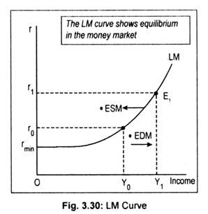
The interest-income combination at which equilibrium occurs, (r₀-Y₀) and (r₁ – Y₁), are points along the LM curve. These points are plotted in Fig. 3.30. Thus, the LM curve is the locus of all combinations of r and Y that bring money market in equilibrium. This LM curve slopes upward to the right because as interest rate rises, equilibrium income rises.

The slope of the LM curve depends on the interest elasticity of money demand. If interest elasticity of money demand is interest- inelastic, the LM curve will be steep and if money demand is assumed to be highly interest-elastic, the LM curve will be flatter.

In an extreme case, if money demand is assumed to be perfectly interest-elastic (it happens at the floor rate of interest or the so- called liquidity trap region), the LM curve also becomes perfectly elastic at this region. In Fig. 3.30 the LM curve is drawn parallel to the horizontal axis at the minimum rate of interest, r_min. The LM curve becomes positively sloped above the r_min range.

Any point off the LM curve shows disequilibrium in the money market. Just to the right of the LM curve there arises excess demand for money (EDM) and to the left of the LM curve excess supply of money (ESM) arises.

Alternative Method of Deriving LM Curve:

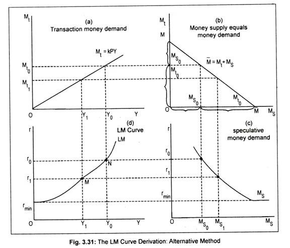
A four-part diagram may be used to derive the LM curve. Fig. 3.31(a) shows a proportional relationship between money income and transaction demand for money (M_t= kPY). Part (c) represents speculative demand for money [M_S = f(r)]. The schedule in (b) is an identity line that mechanically divides money supply into transaction and speculative elements. Part (d) represents the LM curve.

Suppose, the rate of interest, r₀, is known. Given r₀, the volume of speculative demand for money is M_S0. Given the total money sup­ply (M), money not used for speculative pur­poses must be held for meeting transaction demand for money. Thus, the transaction demand for money must be M₁₀. To ensure this transaction demand for money there must be a level of income Y₀. Thus, we see in part (d), for interest rate r₀ the only possible money market equilibrium value for income is Y₀.

If the rate of interest declines to r₁, the equilibrium level of income will be Y₁. The procedure can be repeated such that equilib­rium combinations of r and Y emerge to en­sure equality in the money market. By joining all these combinations (such as, M and N), we get the LM curve drawn in part (d). Note that, at a floor interest rate, r_min, money demand becomes infinitely elastic. This makes specu­lative demand for money (shown in part c) to become horizontal at the minimum rate of in­terest. Because of this liquidity trap, the LM curve also becomes perfectly elastic. Anyway, the LM curve slopes upward from left to right.

Properties of the LM Curve: Summary:

(i) The LM curve consists of equilibrium combinations of income and interest rate for the money market.

(ii) The LM curve slopes upward to the right.

(iii) The slope of the LM curve depends on the interest elasticity of money demand. The LM curve will be (flat) steep if the interest-elasticity of money demand is relatively (low) high.

(iv) The LM curve shifts due to changes in money supply and money demand.

(v) All points on the LM curve show money market equilibrium such that there is neither excess demand money (EDM) nor excess supply of money (ESM). Any point off the LM curve exhibits either EDM or ESM.

A Mathematical Example on the LM Curve:

To derive the mathematical form of the LM equation we consider both money demand and money supply function.

Let transactions demand for money be

M_d = 0.25Y

and speculative demand for money

M_s = Rs. 50 – 200r

Let the money supply be M = Rs. 200

Equilibrium in the money market requires that money supply = money demand

Rs. 200 = Rs. 0.25Y + Rs. 50 – 200r

or 0.25Y = Rs. 150 – 200r

or Y = Rs. 150 + 200r /0.25

= Rs. 600 + 800r is the LM equation.

Given this LM equation, we can find out the level of income if the interest rate is known.

If r = 0.10, then Y = Rs. 680

If r = 0.06, then Y = Rs. 640

By plotting different combinations of r and Y we obtain a positive sloping LM curve.

Practise 1:

Given M_s = Rs. 50 – 400r,

M_t = 0.20Y

and M = Rs. 200.

Find out the LM equation.

Ans. Y = Rs. 750 + 2000r