8 Rules for Finding Derivative of a Function with One Independent Variable

List of eight rules for finding derivative of a function with one independent variable.

Rule # 1. The Derivative of a Power Function:

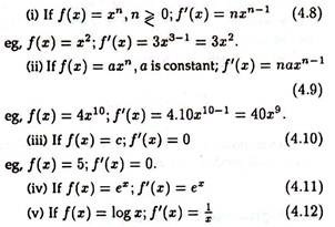
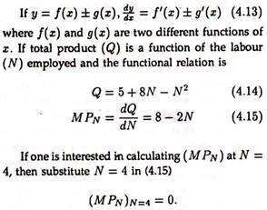
Rule # 2. The Derivative of a Sum or Difference:

Rule # 3. The Derivative of a Product:

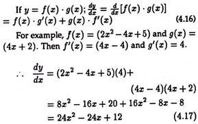
when multiplication of f(x) and g(x) is not tedious, we can first multiply f(x) and g(x) and then apply the derivative of (B).

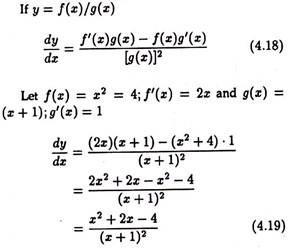
Rule # 4. The Derivative of Quotient:

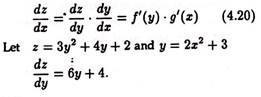
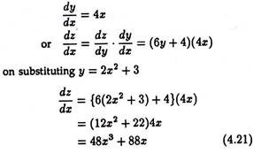
Rule # 5. The Chain Rule:

The rule is also referred to as the function of a function rule, and composite function rule. If we have a given function z = f(y) where y is itself a function of another variable x, denoted by y = g(x), then the derivation of z with respect to x is equal to the derivative of z with respect to y, multiplied by derivative of y with respect to x.

In mathematical notation:

Rule # 6. Partial Differential:

When dealing with different function in Econo­mics, we come across functions where more than one independent variable is involved. For example, the supply function involves many variables-prices, technology, etc. To deal with these types of situa­tions, the concept of partial derivative is every es­sential.

Suppose we consider a function:

z = f(x₁,x₂………………,x_n)

where (x₁………, x_n) are all independent vari­ables. This means that variation in any one of the variables will not affect the other argument of the function. If x₁ changes by Δx₁ and the remaining variables are fixed, the change in z is Δz. Then,

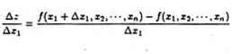
If the limit of Δz/Δx₁ is obtained by allowing Δx₁ → 0, we have the partial derivation. In a similar way, the partial derivations of the other variable can be obtained.

Partial derivatives are written as:

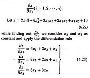
To clarify the situation we take a demand func­tion. Let demand (Q_x) be the function of price (P_x), price of substitute good (P_x) price of complemen­tary good (P_c) and income Y

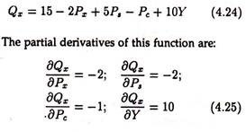
Partial derivatives is equivalent to invoking Ce­teris Paribus assumption that all other variables are held constant. The partial derivation of Q_x with re­spect to Y is 10. This means that quantity demanded increases by 10 unit if income increased by one unit, all other things constant (or Ceteris Paribus). Sim­ilarly, quantity demanded falls by one unit when price of complement (P_c) increases by one unit, Ce­teris Paribus.

Rule # 7. Maximum and Minimum:

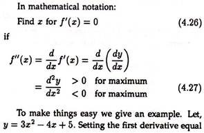
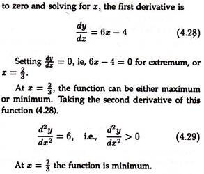
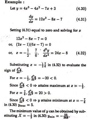
Suppose y = f(x), and f(x) is non-linear, then the value of x for which x is maximum or minimised can be found out by the following rules.

(a) To find the extreme value (maximum or min­imum) of a function, set the first derivative of f (x), i.e., f'(x) equals to zero and solve for x.

(b) The second derivative is the derivative is the first derivative f'(x). The first derivative measures the rate of change of function, the second derivative measures the rate of changes of the derivative func­tion (slope). If the second derivative is negative, it indicates maximum for y\ if it is positive, it indicates a minimum for y.

Rule # 8. Constrained Optimisation:

In the last subsection problems of maximisation and minimisation were dealt with the aid of calcu­lus, but it is to be noted no constraints were in­volved in the process of decision making. In real­ity, however, the management is faced with certain constraints. Some of the problems faced by man­agement are minimisation of cost subject to output constraint or maximising revenue subject to a cer­tain level of profit etc.

Constraints in the form of legal, environment and behavioural act as limiting factors in making decision. In this sub-section we deal with those constraints which can be expressed mathematically and we restrict the number of con­straints to one only. More than one constraint can be taken, but that will make things complicated. To illustrate this, suppose a firm minimise cost and cost function is

C = 10L + 4 K + 300 (4.33)

where L and K denote labour and capital. The pa­rameters 10 and 4 are the unit cost of labour and capital. Now, suppose the management wants to minimise cost subject to level of output (Q) equal to 100 units.

Output is a function of capital and labour defined as:

The firm should use 2√10 and 5√10 units of labour and capital respectively for an output of 100 units. This use of inputs will minimise the cost. To get the minimum cost, we substitute 2 a/5 and 10v^5 for labour and capital in equation (4.33), i.e.,

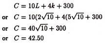
To obtain the minimum cost a lot of substitution has to be done and tackling of the problem becomes more complex when one is faced with more than one constraints. This method is not efficient if one has to face more than one constraint. It that case the technique of Lagrangian multipliers can be applied to tackle problems of constrained optimisation.

The Lagrangian technique combines both the ob­jective function and the constraints. The principle associated with Lagrangian technique is to unconstraint the constrained objective function. The ob­jective function is the cost function is the previous example. A new function is defined which incorpo­rates both the objective function and the constraints with a multiplier termed as Lagrangian multiplier.

Once the hybrid function (combination of objective function and the constraints) termed as Lagrangian function is specified then the next step is to set the partial derivatives equal to zero for all the variables and solve the resulting set of simultaneous equa­tions for the optimal values of the variables.

The Lagrangian multiplier method can be illus­trated by referring to the total cost function intro­duced earlier in this sub-section. The first step is to rearrange the constraints so that all of the terms are on the right hand side of the equation. Thus for total cost function, the constraints becomes.

100-10L^0.5 K^0.5 = 0 (4.36)

Multiplying equation (4.36) by λ (lambda) the unknown multiplier, and adding the result to the total cost function to get the new function.

Z = 10L + 4K + 300 + (100 – 10L^0.5K^0.5) (4.37)

Z is defined as the Lagrangian function. In case of a problem of minimisation, the lambda term should be added in Lagrangian function (and subtracted in the case of a problem of maximisation). The partial derivatives of the Lagrangian function (4.37) are,

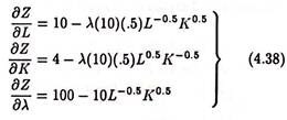
Setting these partial derivative equal to zero, the first order condition, we get

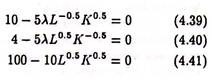
Equation (4.41) is the output constraint. This guarantees that so long as this derivative is zero the constraint conditions imposed upon the original ob­jective function will be satisfied.

Equations (4.39) and (4.40) can be solved for K and L that will minimise the cost of production.

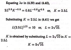
Thus the value of K and L that minimise cost are 5√10 and 2√10 respectively.

The principal advantages of the Lagrangian mul­tiplier technique are that it is easier to apply wher­ever there are multiple constraints. Secondly, this method gives other information of particular impor­tance in the Lagraigian multiplier. In the previous example if we substitute K and L in either equation, (4.39) or (4.40) we can get λ. Substituting K and L in (4.39)

λ = 1.26 (4.42)

The value of λ in general can be regarded as the effect on the objective function of a one-unit change in the constant of the constraining function. In this case the constant of the constraint is out­put of 100 unit and the objective function is cost.

Hence λ — 1.2 denotes the change in cost if output is changed from 100 to 101 unit i.e., λ is the marginal costs. This is a very useful information to manage­ment, regarding changes in cost if output constraint is relaxed.