Empirical Estimation of Demand: Top 10 Techniques

The following points highlight the top ten techniques of Empirical Estimation of Demand. The techniques are: 1. Problems with Theoretical Analysis 2. Estimating Demand Curves 3. The Identification Problem  4. Consumer Surveys 5. Consumer Clinics 6. Market Experiment 7. Multiple Regression Analysis 8. Theoretical Formulation of the Demand Function 9. Regression Analysis of Demand 10. Power Function.

Technique # 1. Problems with Theoretical Analysis:

It is known that demand functions have two im­portant properties:

(1) The demand for any com­modity is a single-valued function of prices and in­come (i.e., a single commodity combination corresponds to a given set of prices and income) and

(2) Demand functions are homogeneous of degree zero in prices and income (i.e., if all prices and in­come change in the same direction and proportion, there is no change in the purchase plan of a consu­mer).

These properties are well established in eco­nomic theory. But the businessman is actually in­terested in having firm knowledge of a portion of the demand curve for the product in which he is in­terested.

It is, of course, possible to estimate the demand function for primary products (e.g., agricul­tural commodities) since data on prices and quanti­ties are readily available for a number of years. But this is not true in the case of manufactured goods.

There is another problem due to the existence of dealers in most markets. Most often than not manu­facturers sell directly to dealers and not to the fi­nal consumers. In the short-run, the whole amount taken by dealers may not be sold to the consumers. The quantities taken by dealers tend to correspond with those taken by consumers only in the long-run.

Moreover, the assumption made in theory that all other factors remain unchanged is unrealistic when we are dealing with market data collected over a number of years. In the long-run, changes in consumers’ incomes, in the size of the population, in the price of related goods and in the conditions of supply, are likely. We have to take note of these realities in estimating the demand for a product.

Technique # 2. Estimating Demand Curves:

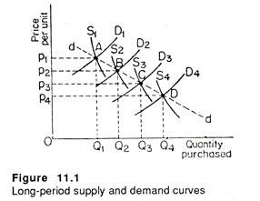
Suppose due to changes in income, population and other factors, the theoretical demand curve shifts from D₁ to D₂, D₂ to D₃ to D₄ in Figure 11.1. The corresponding supply curve at each of these points occupies positions S₁ to S₄. The price-quantity obser­vation which is recorded in period 1 (say, 1981) is given by the intersection of D₁ to S₁, namely, A. The next one is determined by the intersection of D₂ and S₂ at B (in 1982).

Thus we get a series of observa­tions A to D for four years, viz., 1981, 1982,1983 and 1984. These together trace out a demand curve DD. But this is not the same demand curve discussed in theory. More specifically, it is not reversible. It is improbable that we can move back from C to B and B to A.

It is unlikely that the precise combination of conditions which prevailed at these points will be repeated. In practice, the demand and supply curves may not move consistently in the same direc­tion, as is assumed in this diagram. They may move up or down rather erratically.

In Figure 11.1, points A, B and C are not three points on a single demand curve for, say, product X. Each point is on a different demand curve — one that is shifting over a period of time. So just by con­necting them we cannot trace out the product de­mand curve.

A firm may interpret the line dd (which is a Iocus of points A, B, C and D) as the demand curve by mistake. Thus it might assume that a reduction in price from P₁ to P₂ increases sales from Q₁ to Q₂. An expansion of demand may well justify the price re­duction.

But, in practice, such a price cut will result in a much smaller increase in demand. The true de­mand curve (D₁) is much less elastic than the line dd. Thus, a price cut is much less desirable than it appeared at the first sight.

Simultaneous Relationship:

So there is interrelationship between demand and supply curves.

Now, data on prices and quanti­ties purchased can be used to estimate a demand curve only under two sets of conditions:

(1) The de­mand curve has not shifted, but the supply curve has shifted; or

(2) We have almost complete infor­mation to determine just how each curve has shift­ed during the observation period (which covers four years in this case).

Suppose there is a technological change in the production of X. So costs in the industry will fall sharply within a short period but demand condi­tions are likely to be stable. The situation is illus­trated in Figure 11.2. Here the demand curve, which initially was unknown, in now assumed to be stable. The supply curve shifts from S₁ to S₂, S₂ to S₃ and S₃ to S₄.

It is clear that each price/quantity point represents the intersection of the supply and demand curves. Since all the demand determinants except price are assumed to be stable, points A, B, C and D must be on the same demand curve. So the de­mand curve DD can be estimated by connecting the four points.

Technique # 3. The Identification Problem:

It now appears that “the problem of simultane­ous relationships in demand analysis can be over­come only if one has enough information to identify the interrelated functions so that shifts in one curve can be distinguished from shifts in the other.” This is the reason why “the problem of estimating one function when simultaneous relationships exist is known as the identification problem..”

In fact, we must have sufficient information about price/quantity data to separate shifts in de­mand from changes in supply. We may note that in­formation about which curve is shifting and to what extent, is necessary to identity and estimate the demand relationship. This information is not available most of the time.

In practice, some firms do make studies of the influence of price on sales volume, which provides a glimpse of a small section of the demand curve. Most companies rely on the instinct and experience of senior manag­ers with regard to the responsiveness of sales of changes in price.

There is some evidence that busi­nessmen tend to underrate the responsiveness of sales to downward adjustments of price. In such cas­es, statistical demand analysis, with the help of regression technique, is incapable of providing esti­mates of the parameters of the linear demand func­tion.

If it is not possible to solve the identification problem, other techniques such as consumer inter­views and market experiments are used to obtain necessary information about important demand function relationships.

Four primary methods used to estimate the par­ameters (coefficients) of the demand function are: (1) consumer surveys, (2) consumer clinics, (3) mar­ket experimentation, and (4) regression analysis. Regression analysis is perhaps the most important tool of demand analysis for two reasons.

Firstly, in most situations it is perhaps the best, or the only technique of estimating the parameters of the de­mand equation. Secondly, this is perhaps the sin­gle-most important estimating technique used in managerial economics and all other areas of busi­ness administration.

Technique # 4. Consumer Surveys:

Consumer surveys involve questioning a sample of representative consumers to determine such fac­tors as their willingness to buy, their responsive­ness to price changes or to relative price levels and their awareness of advertising campaigns and var­ious other variables considered to be important for the marketing and profit planning functions.

This technique can be applied just by stopping purchas­ers and asking them questions about their inten­tions to buy at different prices. At the other ex­treme, to gather the necessary information, trained interviewers may be appointed to raise sophisti­cated questions to a carefully selected (representa­tive) sample of buyers.

In theory, consumer surveys can provide neces­sary information on the most important demand re­lationships. A firm might question each of its cus­tomers or a sample of customers about projected purchases under a wide variety of conditions relat­ing to price and other factors included in the de­mand function.

Then, by aggregating the data, the firm could forecast its total demand and might be able to arrive at an estimate of some of the impor­tant parameters in the demand function for its product.

Drawbacks:

However, the practical difficulty with this method is that the information obtainable by this technique, and its quality, is likely to be limited. As J. L. Pappas and E. F. Brigham argue, “Consu­mers are often unable, and in many cases unwilling, to provide accurate answers to hypothetical ques­tions about how they would react to changes in the key demand variables”.

For example, most consu­mers are unable to say how they would react to a 1, 2 , or 3% increase (or decrease) in the price of a co­lour T. V. set. This makes if difficult to use such a technique to estimate the demand relationships for most consumer goods.

Merits:

However, there are two advantages of the method. First by using stable inquiries, it is possi­ble for a trained interviewer to extract a good deal of useful information from consumers. For example, an interviewer might ask questions about the rela­tive prices of several pressure cookers or bicycles (which compete closely with one another) and may discover that most people are unaware of existing price differentials.

This is a good indication that demand is inelastic and consumers are not very much price-conscious. So it would not be necessary for a producer to try to cut price to increase demand for its products. Consumers may not even notice the reduction.

Moreover, the effectiveness of advertis­ing campaigns may be tested by sampling the awareness of a group of consumers to the campaign. Thus, it is possible to obtain some basic information through such surveys which may be adequate and reliable for some decision making purposes.

Secondly, there is no substitute of this method for certain kind of information regarding demand for a product. For instance, in short-term demand (or sales) forecasting consumers’ intentions, atti­tudes and expectations about future business condi­tions make all the difference between an accurate estimate and an inaccurate one. It is possible to ob­tain such subjective information through interview methods alone.

For instance, consumer expectations regarding future business and credit facilities may provide significant insights into their propensity to buy many items, especially consumer durables like washing machines, refrigerators, T. V. sets, etc. Moreover, using a little imagination and asking less direct questions may provide substantial in­sights.

Technique # 5. Consumer Clinics:

An alternative means of recording consumer re­sponses to changes in demand determinants is through the use of consumer clinics. This is like a laboratory test in physics or chemistry.

Here ex­perimental groups of consumers are given a small amount of money with which to buy certain items. The experiment can reveal impact on actual pur­chases of the commodity under consideration as its price, prices of competing goods, and other varia­bles affecting demand are manipulated.

Drawbacks:

Although this method is more realistic than the direct interview method, it has two major shortcomings. Firstly, the costs of setting up and running such a clinic are substantial. Consequently, a very small number of consumers can participate in the experiment.

Secondly, since the participants are well aware that their actions are being ob­served, they may behave in a manner somewhat different from normal. This is known as the Haw­thorne effect. A buyer of T. V. set taking part in consumer clinic may suspect that the experimenter is interested in sensitivity to prices and thus may be much more price conscious that he would other­wise be.

However, this approach like the previous one often provides some useful information to the deci­sion-making process. In some situations, this is the only technique that can provide usable informa­tion.

Technique # 6. Market Experiment:

The market experiment method which is often used to gather information about the demand func­tion involves examining the way consumers behave in real life markets. This method involves exami­nation of consumer behaviour in actual markets. Companies may use this method to investigate the nature of their demand curves by experimenting with various prices.

This is also known as market testing. Experiments are made under laboratory condi­tions to derive a demand schedule. Attempts are made “to create the purchasing situation under con­trolled conditions to ensure that price is the only variable”.

Each consumer in the group is offered a choice between the product under investigation and a sum of money, and the number of persons in the group expressing a preference for the product is not­ed.

Then a second group is offered a choice between the product and a different sum of money and the response again noted. By repeating the exercise the number of persons taking the product at different ‘prices’ may be plotted as demand schedule.

This method again has all the defects of the previous method. The consumer has only a choice between the product and a sum of money, whereas in the market he may make choice from competing products. Again, there is no guarantee that the con­sumers will behave under these controlled condi­tions as they do in the market place.

This method also poses difficulties. Firstly, it is necessary in the course of an experiment “to hold non-price factors constant, or at least to provide sta­tistical methods for determining their separate ef­fects. Then, demand may often depend not only on the prevailing price but also on the preceding price”. It is, therefore, difficult to disentangle (i.e., separate out) the effect of the prevailing price from the effect of the price change.

Secondly, competitors something try to inter­fere with market tests by, for example, running spe­cial promotions of their own.

Finally, businessmen often believe that “it is easier to lower price than to raise it. They are therefore, reluctant to experiment with a lower price for fear that, if the experiment is unsuccess­ful, the subsequent price rise will have exception­ally adverse effects”.

Technique # 7. Multiple Regression Analysis:

This is basically a statistical technique. It is used to “isolate” the effects of price from other fac­tors influencing demand. To illustrate, suppose that the Godrej Company hypothesizes that the quanti­ty demanded of its products depends, in addition to price, upon general economic conditions as reflected in the GNP and upon the size of its advertising bud­get.

The assumed relationship can be expressed in the form of an equation where Y represents the de­pendent variable, viz., quantity demanded; X₁, X₂ and X₃ represent the independent variables, viz., price, GNP, and advertising expenditures respec­tively; the coefficients b₁, b₂ and b₃ represent the in­fluence of the respective independent variables on quantity; and the coefficient b₄ is a constant term. The equation is

Y = b₁X₁ + b₂X₂ + b₃X₃ + b₄

If a number of past observations of the independent and dependent variables are available, these ob­servations can be processed statistically to obtain estimates of the co-efficient. The estimated coef­ficient bi, then is taken to represent the influences of price on quantity demanded, other factors being held constant.

In many instances regression analysis is the best, or perhaps the only, means of estimating the de­mand equation.

Technique # 8. Theoretical Formulation of the Demand Function:

The initial step in carrying out a statistical study is to formulate a model based on economic theory. So to start with, we demonstrate how to make use of economic theory by means of mathe­matical tools to formulate a quantifiable statisti­cal model.

The consu­mer’s demand curve for a given commodity can be derived from the analysis of utility maximization. The neo-classical (Marshallian) theory of consu­mer behaviour begins with a utility function that makes an individual’s level of satisfaction de­pend on the commodities he consumes.

Let a consumer’s ordinal utility function be

U = f(q₁, q₂, . . ., q_n) (1)

where q₁, q₂, . . ., q_n are the quantities of different commodities consumed in a single time period. It is assumed that the utility function in Equation (1) is not only an increasing and continuous function of each of the quantities, but is also twice differentiable.

Given the utility function in Equation (1), the theory assumes that consumer behaviour is expli­cable by maximization of Equation (1) with respect to the q’s, subject to budget constraint, namely,

The prices p₁, p₂, . . .,p_n and income y are taken as given to the consumer, and they satisfy the follow­ing conditions:

The maximization of Equation (1) subject to Equation (2) is a constrained maximum problem. A necessary condition for the solution of this type of problem is that

where U_i = (∂U/∂q_i) and λ is the Lagrange multipli­er. In economic terms, λ stands for the marginal util­ity of money. From this it logically follows that

And so on

U_i/P_i = λ, i = 1,2,. . . , n (6)

Thus, in equilibrium, the ratio of the marginal util­ities of two commodities is equal to their price ra­tio, that is, the marginal utilities are proportional to the prices.

Equations (2) and (4) provide (1 + n) relation­ships that permit (1 + n) unknowns, λ and q_i(i = 1,…, n) to be expressed in terms of y and p_i(i =1, …, n). Thus, the solution yields the following demand functions:

q_i = f_i (p₁,p₂,. . . ,p_n,y), i = 1,2,. . . n (7)

In other words, Equation (7) states that consumer demand for the good depends on income and the prices of all commodities.

What is important to note at this stage is that equal proportionate changes in prices and income do not affect the constraint in equation (2) and thus will not affect the utility maximizing values of the q’s. Adopting this property of zero-degree homo­geneity, equation (7) can be written as

where p is an index of general prices. Equation (8) states that the demand for is a function of rela­tive prices of all commodities and real income.

Apart from prices and income, other factors, such as tastes, determine consumer demand. The factors determining preferences, such as family size and composition and residential area, may be noted by x_j, where j = 1, 2, . . ., m. Thus, the demand rela­tionship for an individual consumer may be written in the form

Since the utility function is not measurable in practice, statistical analysis begins directly with the demand functions. The exact functional form is rarely deducted theoretically, but is usually deter­mined empirically (statistically).

Equation (9) is a general function for empirical estimation of a demand function. However, there are several reasons that, in practice, a regression is not specified in a study so as to include all factors that may have causal influence on the dependent variable under analysis. Prima facie it is legiti­mate to make the demand theory as simple as pos­sible, taking into explicit account only the main causal factors.

Secondly, statistical data are lack­ing for certain variables. Furthermore, the causal factors may be highly inter-correlated. Inclusion of a large number of explanatory variables in the model may increase the standard errors of the re­gression coefficients and tend to obscure the impor­tance of explanatory variables in the equation.

Finally, before estimating a demand function empirically, the demand analyst faces an identifi­cation problem. Namely, how do we know that the specified function is not, rather, a supply curve? In other words, how can we distinguish the demand function from the supply function? In fact, the col­lected economic data are already in equilibrium condition where supply is equal to demand.

In spite of these pitfalls we often make regres­sion analysis of demand. The pioneering work in this field was made by T. Schultz in 1938 in the U.S.A., and in 1945 Richard Stone carried out re­gression analysis in the U.K. We may now do re­gression analysis of demand against the backdrop.

Technique # 9. Regression Analysis of Demand:

A frequent objective in business is the specifica­tion of a functional relationship between two vari­ables such as Y =f(X). Here Y is called the depen­dent variable and X the independent variable. In the business world one has to find the relation be­tween sales and advertisement, sales (Y) being the dependent variable and advertisement (X) being the independent variable.

We cannot expect a per­fect explanation of sales by advertisement, and hence we write Y = f(X) + u, where u is a random variable called residual. This is called a regres­sion equation of Y and X. The residual arises from measurement errors in Y , or imperfections in the specification of the function f(X). For example, there may be many other variables beyond X that influence Y, which we have left out.

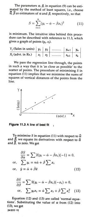
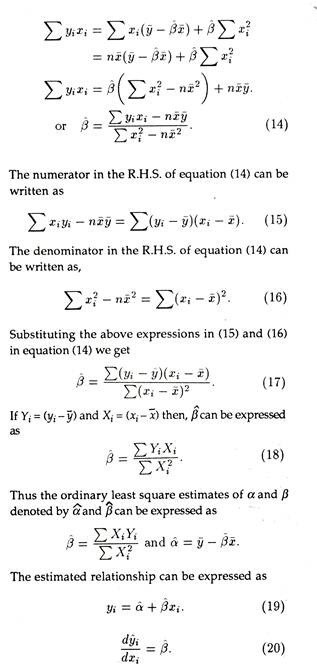
Since u is a random variable, Y is also a random variable. The independent variable X is non- random as fir as business relations are concerned. Assuming f(X) to be a linear function i.e.,f(X) = α + βX., we have

y_i = α + βx_i + u_i i = 1,. . .n (10)

where i = 1, 2, . . ., n denote the number of observa­tions.

The slope coefficient β, gives us an estimate of change in sales associated with a one-unit change in advertising expenditures. The intercept term, α, generally has no economic meaning.

It might be true that the level of sales with zero advertising would equal the intercept term, α, but since there are no observations of sales at zero advertising expendi­tures, we cannot safely assume that α be sales with no advertisement expenditure.

The results of this simple 2-variable regression model can easily be extended to many variables. Suppose that we also have information on the av­erage price p charged for the product. The new in­formation can be added to the linear model in equa­tion (10), resulting in the following regression equation:

Where more than two independent variables are used, we can work out the regression coefficients (in this case β and θ) by matrix method, which is be­yond the scope of the title. Today, the statistical estimation of parameters/coefficients is done by computers. The fitted line is

When this is done, we interpret the coefficients as follows : α is again the intercept term, with little economic significance; β is the expected change in sales related to a one unit change in advertising ex­penditure, holding the price p constant; and θ is the expected change in sales related to a 1-unit change in price, holding advertisement expenditure con­stant. In mathematical notation,

Linear demand functions have great attraction in empirical work for two reasons. First, experience has shown that many demand relationships are in fact linear. Secondly, a convenient statistical tech­nique, the method of least squares, can be used to es­timate the parameters α, β, θ, or the regression co­efficients for linear equations.

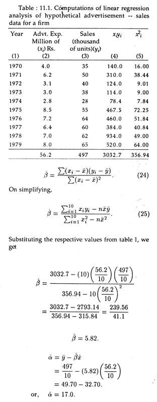
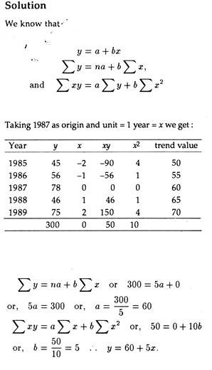
But, this is not the only form of demand function. There can be other forms of demand functions. In the following section we have given an example of how to work out the regression estimates α and β and draw the estimat­ed relation in the case of a linear relation between sales (thousands of units) and advertisement ex­penditure (million of Rs.).

where y_i represents sales and x_i, represents adver­tisement expenditure.

Technique # 10. Power Function:

The second most commonly specified demand re­lationship is the case where two or more interre­lated variable comes into picture. If one assumes constant elasticity’s, power functions can be of use, such as quantity demand Q

P,Y, A are respectively price, income and adver­tisement expenditure. The multiplicative form has a great appeal, since the marginal effects of each of the independent variables depends on the values of other variables in the function.

The marginal impact on the quantity demanded due to change in price will be different for different levels of income (Y) and advertisement expenditure (A). The multi­plicative model described by (27) is in fact more re­alistic than linear functions, where the marginal impact of the independent variables are constant.

The multiplicative model can be made linear by taking logarithmic transformation. Taking log on both sides of equation (27) gives,

log Q = log α + β log P + θ log Y + 7 log A. (28)

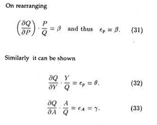
Since the equation is linear in logarithm, one can apply least square regression analysis in estimat­ing the parameters α, β, θ and y. It can be shown that β, θ and y are constant elasticity coefficients.

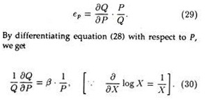
We know that price elasticity of demand is giv­en by the formula

These elasticities, income elasticity of demand (e_y), advertisement elasticity of demand (e_A) and price elasticity of demand (e_p), are constant. The values, θ, y and β are not functions of the variables; for instance, y does not change with changes in P, Q, Y or A.

Constant elasticities are useful where they are appropriate. For example, if income elasticity of demand for television set is constant, then increase in income can be expected to produce proportionate changes in the demand for television over wide ranges of income.

If the income elasticity of de­mand for television set is not constant, then the de­cision maker cannot use the multiplicative model which is beyond the scope of this book. If there are opportunities to employ constant elasticities which may not be frequent, then the multiplica­tive model is very useful because it greatly simpli­fies the analysis.

Example 1

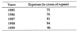
The following table shows the business expen­diture on new plant and equipment i.e., demand for capital goods.

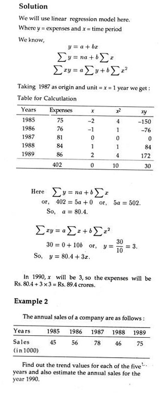
Project the business expenditure on new plant and equipment for the year 1990.