Profit-Maximizing Input Usage

The below mentioned article provides a short notes on Profit-Maximizing Input Usage.

Firms with market power can also reach equilibrium, i.e., their profit-maximizing (or loss-minimizing) position via the selection of the optimal levels of usage of their inputs. To see how this can be made to occur, we may look at the case where the firm employs a single variable input and pays a fixed (constant) price for that input.

One Variable Input with a Fixed Input Price:

Suppose we consider a firm that has market power in its output market it faces a downwards loping demand function for its output. However, the firm is one of many purchasers of the input; so, its employment decision will have no effect on the input price. As an example, one may think of the single electric supply corporation in a city like Chandigarh.

This kind of a firm has substantial market power (albeit in its own small market); so it faces a downward-sloping demand curve. The firm uses one variable input labour in conjunction with its fixed capital stock to produce its output. But, since it is only one of many firms hiring labour in the city, its employment decision how many workers it hires is unlikely to exert any influence on the city-wide wage rate.

We know that the optimum level of employment for the firm is that at which the MRP is equal to the price of the input:

MRP_L= w

where MRP_L is the marginal revenue product of labour and w is the market-determined wage rate. We also know that, for a firm with market power, MRP is equal to the product of the firm’s marginal revenue function and the marginal physical product function for the input:

MRP_L = MR x MPP_L

Again we may use a one-input (short-run) production function of the form Q = AL_β

where 0 < β < 1. As we know, the marginal physical product function for labour is

MPP_L = β AL ^β-1

Here we also use a log-linear demand function

Q = P^b Y^c P^d_R

After estimating this demand function statistically and obtaining forecasts for the exogenous variables Y and P_R — the forecasted demand function may be written as

Q = BP^b

and the marginal revenue function as

MR =(b+1/b)B –1/b Q1/b

If, however, we want to solve for the optimal level of usage of labour, the marginal revenue function has to be expressed in terms of L rather than Q. This is done by substituting the production function (Q = AL^β) into our MR function to get:

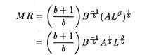
We obtain the marginal revenue product function as

MRP_L = MR X MPP_L

where the MR and MPP_L functions are those derived above. Then, to determine the optimal level of usage of labour, we have to equate this marginal revenue product function to the price of labour, w, and solve for L.

Monopsony:

We have looked at competitive and monopolistic firms demanding labour in competitive labour markets, but now we want to consider the case where there is market power in the labour markets. We have assumed to this point that the purchasing firm had no effect on wage rates.

But what if the firm does affect wage rates, so that as the firm hires more labour, the wage rate rises? We refer to such a firm as having monopsony power. Pure monopsony is the case of a single purchaser of a particular input.

Let’s consider first the case of pure monopsony. We will begin by assuming that a firm’s MRP_L curve is known to us, as in Figure 16.8. The market supply curve of labour to this firm, S_i, is known to us. Table 16.3 provides a numerical example of the monopsony supply curve. The market supply curve, S_L, is the supply curve the firm faces because the firm is the market for this class of labour by the definition of monopsony.

If this were a competitive market, a wage rate of OW_c and employment of OL_c would have resulted. However, since the firm faces the upward sloping supply curve, S_L the marginal resource cost curve for labour (MFC_L) lies above the S_L curve, as in Figure 16.8. To see why this is the case refer to Table 16.3.

The supply curve is, of course, the graphical representation of columns 1 and 2. Since the curve is upward sloping, the firms must pay a higher wage rate as it hires extra workers. Consequently, total wage expenses (column 3) increase.

The amount that each additional labour unit hired adds to wages expenses is the marginal wage cost, or the marginal factor cost of labour. By comparing columns 2 and 4 we see that the curve representing column 4 will lie above the supply curve, as shown in Figure 16.8.

The firm, as before, maximises profits where MRP_L = MFC_L. This would be at point A on Figure 16.8. So the firm employs OL_m units of labour. But what is the wage rate? The supply curve tells us what has to be paid to hire OL_m units of labour L. So the firm will pay OW_m. Note, the OW_m < OW_c, so the monopsonist is paying a lower wage than that would have been paid in a competitive labour market.

Mrs. Joan Robinson refers to this situation as monopsonistic exploitation because labour is receiving less than a competitive wage. This does not mean that workers are forced to work at wage rates below what they are willing to work for. Rather, the monopsony simply restricts input to depress wages and exploits the workers.