How to Derive Demand Theorem from Revealed Preference Hypothesis?

Revealed preference hypothesis can be utilised to establish the demand theorem.

Samuelson has derived the Marshallian law of demand from his revealed preference hypothesis.

Marshallian law of demand, as is well known, states that a rise in the price of a good must, if income and other prices are held constant, results in the reduction of amount demanded of the good, and vice versa.

In other words, according to Marshall’s law of demand, there is inverse relation between price and amount demanded of a good. Samuelson proceeds to establish relationship between price and demand by assuming that income elasticity of demand is positive. From positive income elasticity, he deduces the Marshallian inverse price-demand relationship.

He states the demand theorem what he calls the Fundamental Theorem of Consumption Theory as under:

“Any good (simple or composite) that is known always to increase in demand when money income alone rises must definitely shrink in demand when its price alone rises”.

Fundamental Consumption Theorem and Rise in Price:

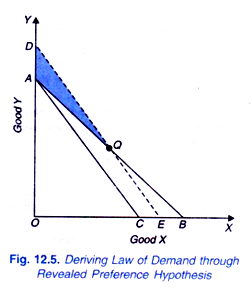
It is clear from the above statement of Fundamental Theorem that positive income elasticity of demand has been made a necessary qualification to the inverse price-demand principle. The geometrical proof of the Fundamental Theorem is illustrated in Fig. 12.5. Let us suppose that the consumer spends his entire income on the two goods X and Y.

Further suppose that his income in terms of good X is OB, and in terms of good Y is OA. Now, the price line AB represents the price-income situation confronting the consumer. All the combinations of goods X and Y lying within or on the triangle OAB are available to the consumer, from which he can buy any combination. Suppose that the consumer is observed to choose the combination Q. This means that Q is revealed to be preferred to all other combinations that lie within or on the triangle OAB.

Now, suppose that the price of good X rises, his income and price of Y remaining unchanged. With the rise in price of X the price line shifts to the new position AC. The price line AC represents new price-income situation. We now want to know what is the effect of this rise in price of good X on its quantity demanded, assuming that demand varies directly with income (i.e., income elasticity of demand is positive).

It is evident from Fig. 12.5 that combination Q is not available to the consumer in price-income situation AC. Let us compensate the consumer for the higher price of X by granting him extra money so that he can buy the same combination Q even at the higher price of X. The amount of money which is required to be granted to the consumer so that he could buy the original combination Q at the higher price of X has been called Cost-difference by J. R. Hicks. In Fig. 12.5. a line DE parallel to AC has been drawn so that it passes through Q. DE represents higher price of X and the money income after it has been increased by the cost difference.

Now, the question is which combination will be chosen by the consumer in price-income situation DE. The original combination Q is available in price-income situation DE. It is evident from Figure 12.5, that he will not choose any combination lying below Q on the line DE. This is because if he chooses any combination below Q on the line DE, his choice would be inconsistent.

All combinations below Q on DE, that is, all combinations on QE could have been bought by the consumer but had been rejected by him in price-income situation AB in favour of Q. (All points on QE were contained in the original choice triangle OAB.). Since we are assuming consistency of choice behaviour on the part of the consumer he will not choose, in price-income situation DE, any combination below Q on QE in preference to Q when Q is available in the new situation.

It follows, therefore, that in the price-income situation DE the consumer will either choose the original combination Q or any other combination on QD portion of DE or any combination within the shaded area QDA. (It should be noted that choice of any other combination on QD or within the shaded area QDA in preference to Q by the consumer will not be inconsistent since combinations lying above Q on QD or within the shaded region QDA were not available in price-income situation AB.)

In price-income situation DE if the consumer chooses the original combination Q, it means he will be buying the same amount of goods X and Vas before, and if he chooses any combination above Q on QD or within the shaded area QDA, it means that he will be buying less amount of commodity X and greater amount of Y than before.

Thus, even after sufficient extra income has been granted to the consumer to compensate him for the rise in price of good X, he purchases either the same or the smaller quantity of X at the higher price. Now, if the extra money granted to him is withdrawn, he will definitely buy the smaller amount of X at the higher price, if the demand for good X is known always to fall with the decrease in income (that is, if income elasticity of demand for X is positive).

In other words, when the price of good X rises and no extra money is granted to the consumer so that he faces price-income situation AC, he will purchase less amount of good X than at Q. Thus assuming a positive income- elasticity of demand, the inverse price-demand relationship is established through revealed preference hypothesis so far as rise in price is concerned.

Proving Consumption Theorem in Case of fall in Price:

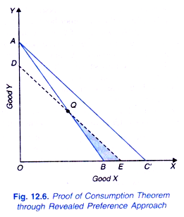
That the inverse price-demand relationship holds good in case of a fall in price also is demonstrated in Fig. 12.6. Let us suppose that AB represents original price income situation and further that the consumer reveals his preference for Q over all other combinations within or on the triangle OAB. Now, suppose that price of good X falls so that the price line shifts to the right to the position AC.

Let us take away some amount of money from the consumer so that he is left with just sufficient amount of money which enables him to purchase the original combination Q at the lower price of good X. Thus, in Figure, 12.6, a line DE is drawn parallel to AC so that it passes through Q. Price line DE represents lower price of X as given by AC and the money income after it has been reduced by the cost difference.

It is obvious that in price-income situation DE, the consumer cannot choose any combination above Q on QD, since all such combinations were available to him in the original price-income situation AB and were rejected by him in favour of Q. The consumer will, therefore, choose either Q or any other combination on QE or from within the shaded region QEB.

In price-income situation DE, his choice of Q means that he buys the same quantity of goods X and Y as in original price-income situation AB, and his choice of any other combination on QE or from within the shaded region QEB means that he buys larger amount of good X and smaller amount of good y than in the original price-income situation AB.

Thus, even after consumer’s income has been reduced, he buys either the same quantity of X or more at the lower price. And if we give him back the amount of money taken away from him so that he confronts price-income situation AC’ he will definitely buy more of X at the lower price, provided that his demand for X rises with the rise in income (i.e. his income elasticity of demand for good X is positive).

The two demonstrations given above together prove the fundamental theorem of consumption theory, according to which any good whose demand varies directly with income must definitely shrink in demand when its price rises and expands in demand when its price falls. It may be noted that Samuelson’s theory involves two implicit assumptions which have not been explicitly stated. In the first place the consumer is always shown to choose a combination on the budget line.

In other words he is never shown to choose a combination from within the triangle. This is based upon the assumption that a consumer always prefers a larger collection of goods to a smaller one. Secondly, another implicit assumption involved in Samuelson’s theory is that the consumer is shown to choose only one combination of goods in every price-income situation. With these two implicit assumptions the inverse price-demand relationship is deduced by Samuelson by making explicit assumptions of consistency of choice and a positive income- elasticity of demand.

Breaking up Price Effect into Substitution Effect and Income Effect:

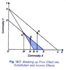
Having now explained the derivation of law of demand from revealed preference approach we are now in a position to show how in the revealed preference approach price effect can be broken up into substitution and income effects. We will explain this by considering the case of fall m price of a commodity. Now consider Figure 12.7 where, to begin with, price income situation faced by a consumer is given by the budget line AB. With price income situation represented by the budget line AB, suppose the consumer chooses combination Q and buys OM quantity of commodity X.

Now, suppose price of commodity X falls and as a result budget line shifts to the new position AC. Now, income of the consumer is reduced so much that the new budget line DE passes through the original chosen combination Q. That is, income is reduced equal to the cost difference so that gain in real income caused by the fall in price of commodity X is cancelled out.

As seen above, with the new budget line DE, to be consistent in his behaviour the consumer can either choose the original combination Q or any combination lying on the segment QE of the budget line DE or from within the shaded area QEB. If he chooses again the original combination Q, the Slutsky substitution effect will be zero. However, suppose that the consumer actually chooses combination S on the segment QE of the new budget line DE.

Now, choice of the combination S shows that there will be substitution effect due to which the consumer will buy MN more of good X. Note that substitution effect is negative in the sense that the relative fall in price of good X has led to the increase in quantity demanded of X, that is, change in quantity demanded is in opposite direction to the change in price.

It should be noted that choice of combination S on segment QE in preference to combination Q of the budget line DE is not inconsistent because combinations on QE segment and within the shaded area QEB were not available before when combination Q was earlier chosen in price-income situation AB.

Thus, with the new budget line DE after consumer’s income has been adjusted to cancel out the gain in real income resulting from a relative fall in price of X, the consumer chooses either Q (when substitution effect is zero or a combination such as S on segment QE when substitution effect leads to the increase in quantity demanded of good X by MN.

This is generally known as Slutsky theorem which states that if income effect is ignored substitution effect will lead to the increase in quantity demanded of the good whose price has fallen. Therefore, according to Slutsky theorem, due to the negative substitution effect, the Marshallian law of demand describing inverse relationship between quantity demanded and price of a good will hold good, that is, due to substitution effect alone demand curve slopes downward.

Now, if the consumer chooses the combination S on the line segment QE of budget line DE, it means that he buys MN more due to the substitution effect. Thus he prefers combination S to combination Q. In other words, his choice of S instead of Q reveals that he will be better off at S as compared to Q. Now, if money income withdrawn from him is restored to him so that he is faced with the budget line AC.

If income effect is positive, he will choose a combination, say R, on the budget line AC to the right of point S indicating that as a result of income effect he buys NH more of the commodity X Thus quantity demanded of commodity X increases by MN as a result of substitution effect and by NH as a result of income effect. This proves the law of demand stating inverse relationship between price and quantity demanded.

On budget line DE, if the consumer chooses combination Q and consequently substitution effect is zero, the whole increase in quantity demanded MH as a result of decline in price of good X will be due to positive income effect. However, it is more likely that the substitution effect will lead to the choice by a consumer a combination such as S that lies to the right of Q on the line segment QE and will therefore cause increase in quantity demanded. This substitution effect is reinforced by the positive income effect and as result we get a downward-sloping demand curve.

It needs to be emphasised that in revealed preference theory it is not possible to locate exact positions of points S and R obtained as a result of substitution effect and income effect respectively. It will be recalled that with indifference curve analysis we could obtain precise points to which a consumer moves as a result of substitution and income effects and these were the points of tangency of indifference curves with the relevant budget lines.

As explained above, revealed preference theory is based on the assumption that all points on or below the budget line are strongly ordered and relation of indifference of a consumer between some combinations of goods is therefore ruled out. In revealed preference theory, choice of a consumer reveals his preference for a chosen position; it cannot reveal indifference of the consumer between combinations.

Therefore, in revealed preference theory we can only say about the direction of substitution effect through logical ordering and cannot measure the exact size of it, nor we can measure the exact amount of income effect of the change in price.

Besides, the substitution effect obtained through variation in income through cost difference method, does not represent pure substitution effect in the Hicksian sense in which the consumer’s satisfaction remains constant. In substitution effect obtained by the revealed preference theory through Slutskian method of cost difference, the consumer moves from point Q to point S on budget line DE.

His choice of S on budget line DE instead of Q under the influence of substitution effect shows that he prefers S to Q. That is, he is better off in position S as compared to the position Q. Therefore, it is maintained by some economists that the substitution effect obtained in revealed preference theory is not a pure one and contains also some income effect.

However, the present author is of the view that the two types of substitution effect (Hicksian and the one obtained in revealed preference theory) differ with regard to the concept of real income used by them. In indifference curve analysis the term real income is used in the sense of level of satisfaction obtained by the consumer, whereas in revealed preference theory real income is used in the sense of purchasing power.

Thus, Hicksian substitution effect involves the change in the quantity demanded of a good when its relative price alone changes, level of his satisfaction remaining the same. On the other hand, revealed preference theory considers substitution effect as the result of change in relative price of a good on its quantity demanded, consumer’s purchasing power remaining the same.

In Fig. 12.7. when we obtain budget line DE after reduction in income by the cost difference so that it passes through the original combination Q chosen by the consumer before the fall in price. This implies that with budget line DE, he can buy, if he so desires, the original combination Q that is, the gain in purchasing power or real income caused by fall in price of X has been cancelled out by the reduction in his money income.