The Model of Aggregate Demand and Supply (With Diagram)

Let us make an in-depth study of the Model of Aggregate Demand and Supply. After reading this article you will learn: 1. Introduction to the Model 2. Aggregate Demand 3. Shifts in the AD Curve 4. Aggregate Supply 5. The Long-Run Vertical AS Curve 6. The Horizontal Short-Run AS Curve 7. Short-Run Equilibrium of the Economy 8. The Long-Run Price Adjustment 9.Comparison of the Two Types of Intertemporal Adjustment.

Introduction to the Model:

In the classical model the amount of output depends on the economy’s ability to supply goods and services, which, in its turn, depends on three things: (i) existing stock of capital, (ii) labour force and (iii) unchanged technology.

According to the classical theory, price flexibility ensures full employment.

The theory is based on the fundamental proposition that price adjusts to ensure that the quantity of output demanded and the quantity supplied are always in balance.

However, in a world of sticky prices, output also depends on the demand for goods and services. Aggregate demand is influenced mainly by demand management (monetary and fiscal) policies. Such policies can exert influence on the economy’s output in the short run when prices are sticky.

This is why such policies can stabilises the economy in the short run. In the long run money has a neutral effect on the real variables because prices are variable but aggregate output is sticky.

Aggregate Demand:

The term aggregate demand (AD) is used to show the inverse relation between the quantity of output demanded and the general price level. The AD curve shows the quantity of goods and services desired by the people of a country at the existing price level. In Fig. 7.2 the AD curve is drawn for a given value of the money supply M.

The AD curve is downward sloping for two reasons:

(i) The fall in the quantity of goods and services purchased:

Since the velocity of money is assumed to remain constant, the ex­isting stock of money determines the rupee value of all transactions in the economy (as has been postulated by the quantity theory of money.) if the price level rises, more money is required to carry out each transaction.

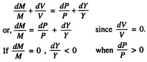
This means that the number of transactions and thus the quantity of goods and services has to fall. Since MV= PY and V = V, a rise in P implies a fall in Y, since M determines PY. If M = M, a rise in P implies a fall in Y. We know that

(ii) Real balance effect:

A rise in the price level implies a fall in the level of real balances (M/P). This, in its turn, implies a smaller quantity of goods and services. In other words, if Y increases, people engage in more transactions and need higher real balances. For a fixed supply of M, higher real balances imply a lower price level. The converse is also true.

Shifts in the AD Curve:

The AD curve shows alternative feasible combinations of P and Y for a given value of M. If the central bank changes M, then the possible combinations of P and Y change, too and the AD curve shifts. The AD curve also shifts at a fixed value of M if V changes.

If the central bank reduces M, there will be a proportionate fall in PY (the nominal value of output). If P remains fixed, Y will fall and, for any given amount of Y, P is lower. In this case the AD curve showing inverse relation between P and Y shifts to the left from AD₁ to AD₂ in Fig. 7.3. Fig. 7.3 also shows that the AD curve shifts to the right in case of an increase in M by the central bank.

Aggregate Supply:

The aggregate supply (AS) is the relationship between the quantity of goods and services supplied and the price level. However, the shape of the AS curve depends on the behaviour of prices which, in its turn, depends on the time horizon under consideration.

The Long-Run Vertical AS Curve:

Since output does not depend on the price level in the classical model, which takes a long-run view of the economy the AS curve is vertical as shown in Fig. 7.4. In the long run aggregate supply (AS) depends on capital, labour and existing technology and is specified by the aggregate production function Y = F (K̅, L̅) = Y̅.

In such a situation changes in AD affect the price level, but not output. However, if M falls the AD curve shifts to the left and the price level falls as shown in Fig. 7.5, output remaining constant at Y̅.

The vertical LRAS curve proves the validity of the classical dichotomy that Y (a real variable) is independent of M. The long-run level of output, Y̅, is called the natural level of output or full employment output, at which actual employment is at its natural rate and cyclical unemployment is zero.

The Horizontal Short-Run AS Curve:

Since prices remain fixed in the short run the AS curve is horizontal. The reason for price rigidity is that all prices remain fixed at some predetermined levels and firms adjust their output levels by hiring enough labour to meet the existing demand for goods and services at these prices.

Short-Run Equilibrium of the Economy:

In the short run the economy reaches equilibrium at the point where SRAS curve intersects the AD curve as at point E in Fig. 7.7. Since the SRAS curve is horizontal, changes in AD lead to changes in aggregate output. If, for example, the AD curve shifts to the left due to a fall in the money supply, aggregate output falls from Y₀ to Y₁ the aggregate price level remaining the same as shown by a movement of the economy from point E to E’ along the SRAS curve.

A fall in AD leads to a fall in Y at a fixed P. So the economy experiences a recession, which refers to a period of high prices and low demand. Due to sticky prices, a fall in demand leads to a fall in production, and a fall in employment (or an increase in unemployment). In the short run price stickiness is the cause of unemployment. (Price flexibility does not ensure automatic full employment in the long run as in the classical model.)

The Long-Run Price Adjustment:

In the long-run prices are flexible, as in the classical model and actual output is equal to the potential (full employment) level. In such a situation a fall in AD will cause only P to fall, with Y remaining constant. The long-run equilibrium of an economy is at point E in Fig. 7.8 where the AD curve intersects the LRAS curve.

Due to price adjustment in the long run, the SRAS curve also passes through point E. In other words, as prices are adjusted to reach long-run equilibrium, when the economy is at point E, the SRAS curve must intersect the LRAS curve.

Comparison of the Two Types of Intertemporal Adjustment:

In Fig. 7.9 we make a comparison between the adjustment of the economy in the short run and in the long run. In the short run a fall in aggregate demand and a shift of the AD curve to the left from AD₁ to AD₂ leads to a fall in output from Y̅ to Y_a, as is shown by points E and E.

But in the long run when output is at its natural level, a fall in aggregate demand leads to a fall in the price level from P̅ to P_a, as is seen by comparing points E and E. In short, a fall in aggregate demand in the short run leads to a fall in output but in the long run output returns to its normal level due to price adjustment by the firms.