3 Main Types of Price Effect (PE)

The following points highlight the three main types of price effect on the quantity demanded for a commodity. The types are: 1. Normal Good 2. Non-Giffen Inferior Good 3. Giffen-Inferior Good.

Price Effect: Type # 1. Normal Good:

The effect on the quantity demanded of a change in its own price is called the price effect. This shows the total effect of price change. Change in price, in general, exerts two influences on quantity demanded. These two are:

Income effect (IE), and the substitution effect (SE).

In the first place, when the price of X’ falls the real income (purchasing power) of the consumer goes up. A consumer thinks that his real income has gone up but money income is held constant. With the increased real income the consumer can purchase more of a commodity—this is the income effect of price change which may be positive or negative.

If the consumer purchases more of a commodity following an increase in real income (due to a fall in the price of commodity) income effect is said to be positive. It will be negative when a consumer purchases less of a commodity following a fall in real income.

Secondly, when the price of a commodity falls, the relative price changes. When price of ‘X’ falls, X becomes cheaper and Y dearer. A consumer will always prefer cheaper commodity for dearer commodity. This is known as the substitution effect.

The substitution effect, thus, reflects the tendency for a consumer to substitute one good for another when there is a change in the relative price of two goods. The substitution effect measures the effect of changes in relative price of any commodity, holding the real income constant.

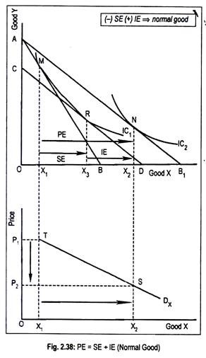
By constancy in real income we mean that the money income and the relative prices are so changed that the consumer stays on the same indifference curve, thereby giving the same level of satisfaction after the change in price. Thus the price effect (PE) is the result of two effects—the income effect and the substitution effect. These two effects of a fall in price can now be explained in terms of Fig. 2.38.

In Fig. 2.38, AB is the initial budget line and M is the initial point of equilibrium. Corresponding to this equilibrium point, our consumer purchases OX₁ of X. Now the price of X falls and the budget line shifts to AB _x which is tangent to the higher indifference curve IC₂ at point N. As a result of this, the consumer buys more of X. Thus, the movement from M to N is to be called the price effect, or in quantitative terms, it is X₁X₂.

Now this price effect can be decomposed into income effect and substitution effect. In order to separate them we remove the influence of the rise in real income caused by the price change. We know that when the price of a commodity falls the real income of the consumer goes up.

If this increased real income is taxed away the budget line AB₁ will shift parallel to the downward direction, so that relative prices are kept at their new level. Here the money income of the consumer is so reduced that the gain in real income due to a fall in the price of X is eliminated.

The relative price is no longer given by the slope of the line AB but by the slope of the line CD. We have drawn the imaginary budget line CD parallel to AB₁. The budget line is thus shifted to the left in such a way that it is tangent to the initial indifference curve IC₁ at R.

The movement from M to R along the same indifference curve, IC₁, measures the substitution effect of price change. Here, as X is cheaper and Y is dearer, the consumer buys more of X and less of Y. Thus, in quantitative terms, X₁X₃ is the substitution effect.

Substitution effect is always negative due to which the consumer buys more of X when its price falls.

Now, we return the consumer’s increased money income which had been taxed away earlier. The budget line shifts parallel to AB₁ and the consumer climbs up to a higher indifference curve IC₂ and equilibrium occurs at point N. The movement from R to N is, thus, the income effect which enables the consumer to buy more of X, that is, X₃X₂. Here, the price effect is negative.

As per our diagram:

PE = X₁X₂

SE = X₁X₃

IE = X₃X_2.

X₁X₂ = X₁X₃ + X₃X₂

Generally, these two effects operate in the same direction, so that a fall in the price of a commodity causes the consumer to buy more of it. In other words, as positive income effect and negative substitution effect work in the same direction, demand for X rises when its price falls. Here, X is a normal good or a superior good since the income effect is positive.

Demand curve for a normal good has been drawn in the lower panel of Fig. 2.38. Let us assume that the initial price of X is OP₁ in accordance with the original budget line AB. At this price, the consumer buys OX₁. When the price of X drops to OP₂ the budget line shifts to AB₁. Quantity demanded rises to OX₂. Now, by joining the points T and S, we get a negative sloping demand curve. Thus, X is a normal good.

PE = SE + IE:

Price Effect: Type # 2. Non-Giffen Inferior Good:

In the case of an inferior good, income effect is negative since demand for it tends to decline as income rises. However, the substitution effect for any good is always negative.

Thus, for an inferior good, both income effect and substitution effect are negative but negative substitution effect outweighs negative income effect. That is why demand curve for an inferior good is also negative sloping, rather than positive sloping. In other words, inferior good (defined in this sense) is not a Giffen good.

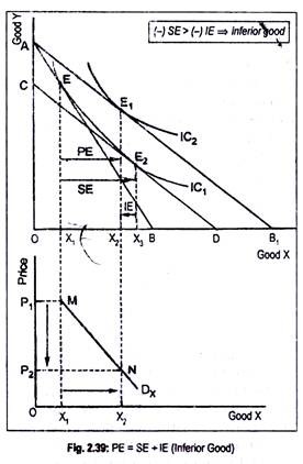
In Fig. 2.39 we show the income effect and substitution effect of a price change for an inferior good. AB is the initial budget line and IC₁ is the initial indifference curve. E is the initial equilibrium point. At this point, our consumer buys OX₁ of X and EX₁ of Y.

Now, suppose the price of X is reduced such that the budget line shifts to AB₁ and the consumer reaches equilibrium at point E₁ on IC₂. The total price effect is, thus, X₁X₂ which can be split into substitution effect and income effect.

To examine the substitution effect first, we have drawn an imaginary budget line CD in such a way that it touches the initial indifference curve (IC₁) so that satisfaction remains unchanged. This occurs at point E₂. Thus, the movement from E to E₂ along the same indifference curve is the substitution effect, or in quantitative terms, X₁X₃.

The movement from E₂ to E₁ describes income effect. [If an income consumption curve is drawn, it will take a backward turn]. Income effect is, thus, negative, since quantity demanded has decreased from OX₃ to OX₂. Since income effect is negative, the product in question is an inferior one.

Thus, PE = X₁X₂

SE = X₁X₃

IE = X₃X₂

Because of negative substitution effect, quantity demanded should rise while quantity demanded should decrease because of negative income effect. However, negative substitution effect outweighs negative income effect. That is why quantity demanded rises as price falls. The lower half of the figure shows that, as the price of X falls from OP₁ to OP₂, quantity demanded rises from OX₁ to OX₂.

Therefore, for an inferior good, demand curve is also negative sloping. The only difference in the nature of the negatively sloped demand curve for normal or superior good and inferior good is that demand for an inferior good is relatively less elastic.

PE = SE + IE:

Price Effect: Type # 3. Giffen-inferior Good:

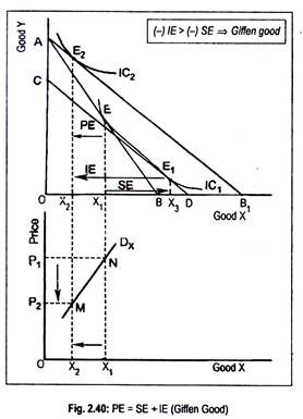
Since income effect is negative, Giffen good must be an inferior good. But for a Giffen- inferior good, negative income effect is more strong than the negative substitution effect. As a result, demand for a Giffen good rises (falls) when its price rises (falls). In other words, 4emand curve becomes positive sloping. This is shown in Fig. 2.40.

According to this figure,

PE = X₁X₂

SE = X₁X₃

IE = X₃X₂

As usual, the substitution effect (i.e., the movement along the same indifference curve) is negative and is measured by the distance X₁X₃. Negative substitution effect causes quantity demanded to rise (fall) when price falls (rises). Here, the commodity is an inferior one since income effect is negative. It is due to the negative income effect that quantity demanded falls (rises) when real income rises (falls).

Note that the negative income effect is more strong than the negative substitution effect. Hence, the good is a Giffen-inferior one. Anyway, demand curve is, thus, positive sloping. As price falls, demand falls and, as price rises, demand rises.

Remember that all Giffen goods are inferior goods but all inferior goods are not Giffen goods. Inferior good is an income phenomenon while Giffen good is a price phenomenon that violates the law of demand. In fact, Giffen good, not an inferior good, is a bona fide exception to the law of demand.