
In this article we will discuss about the demand function for exports.
The responsiveness of the demand for Exports to the changes in the real world income and the ratio of unit value of exports of a country price to the unit value of world price [Relative price] variable can be estimated by OLS method using time series data.
Demand function for Exports can be specified as follows:
Y = f (X1, X2)
ADVERTISEMENTS:
Where
Y = Quantity of country’s aggregate exports
X1 = Real world income
X2 = Relative price variable [Unit value of exports/world price level]
ADVERTISEMENTS:
Partial elasticity of demand for exports with respect to Real World Income, all else equal
eY.X1 = dY/dX1 * X1/Y > 0
Partial elasticity of demand for exports with respect to relative price level, all else equal
ey.x2 = dY/ dX2 * X2/Y ![]() 0
0
Demand function for exports will be estimated by fitting the linear and log linear regression models to the time series data.
ADVERTISEMENTS:
Linear Demand Function for Exports:
The specification of a linear demand function for exports will be as follows
Y = b0 + b1X1 + b2X2 + error……………….. (35)
Partial derivative of Y with respect to X1, ∂Y/∂X1, b1, explains the rate rate of change in Y per a unit change in real world income.
Partial derivative of Y with respect to Relative Price, ∂Y/∂X2, is b2, which shows the rate of change in Y per a unit change in Relative Price. Both b1 and b2 are constants i.e., they are independent of changes in World Real Income and Relative Price. Elasticities of demand for Exports with respect to World Real Income and Relative Prices will be evaluated from the linear regression model.
Partial elasticity of demand for exports with respect to real world income will be estimated as follows
ey.x1 = ∂Y/∂X1. X1/Y = b1X1/Y
The elasticity will be evaluated from point to point change in X1 and Y. But in the empirical studies, the elasticities are being evaluated at the mean values of X1 and Y. Hence they are called average elasticities of demand for exports.
ADVERTISEMENTS:
ey.x1 = ∂Y/∂X1. X1/Y = b1 mean of X1/mean of Y
If its value is greater than unity then the proportionate change in Y, will be relatively higher than the proportionate change in Real World Income. If it is less than one then the proportionate change in Y will be relatively lower than the proportionate change in Real World Income. If it is unity, then the proportionate change in Y will be equal to the proportionate change in X1.
Partial Elasticity of K with respect to Relative Price will be estimated as follows
ey.x2 = ∂Y/∂X2. X2/Y = b2. X2/Y,
ADVERTISEMENTS:
This elasticity will also be evaluated from point to point change in X2 and Y. In empirical studies the elasticities of demand for exports are evaluated at mean values of X2 and Y.
ey.x2 = ∂Y/∂X2. X2/Y = b2. mean of X2/mean of Y
If its value is greater than 1, then the proportionate change in Y will be relatively higher than the proportionate change in relative price. If it is less than 1, then the proportionate change in Y will be relatively smaller than the proportionate change in relative price.
If it is unity then the proportionate change in Y will be equal to the proportionate change in relative price. The reliability of these elasticities will be evaluated on the basis of statistical significance of b1 and b2. If the linear demand function for exports fitted to time series data is not suited, then other forms of equations have to be tried.
ADVERTISEMENTS:
Log Linear Demand Function for Exports:
The most commonly used form of regression model [Equation] for estimating the income and price elasticities of demand for exports is the Power function [Which is also known as the log linear regression model if specified by taking logarithms] whose specification will be as follows:
Y = b0X1b1 X2b2 ……………………….(36)
The partial derivative of demand for exports with respect to World Real Income is,
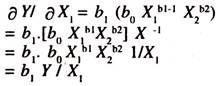
ADVERTISEMENTS:
The partial constant elasticity of demand for exports with respect to World Real Income is
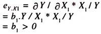
ADVERTISEMENTS:
The partial derivative of demand for exports with respect of Relative Price is
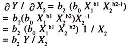
ADVERTISEMENTS:
The partial constant elasticity of demand for exports with respect to World Real Income is
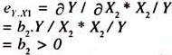
ADVERTISEMENTS:
Thus, the partial derivatives are not independent of changes in Y, X1 and X2 i.e., they go on changing, with the change in Y, X1 and X2 and the partial elasticities of demand for exports are constants.
For the purpose of estimation, the power function is transformed into a log linear function as shown below:
log Y = log b0 + b1 log X1+ b2 log X2 ………………..(37)
The partial derivative of log Y with respect to log X1 [Which is the partial elasticity of demand for exports with respect to World Real Income] is
∂ log Y/ ∂ log X1 = ∂ Y/Y/ ∂ X1/X1 = ∂ Y/ Y. X1 /∂ X1 = b1
The partial derivative of log Y with respect to log X1 [Which is the partial elasticity of demand for exports with respect to relative price] is
∂ log Y/ ∂ log X2 = ∂ Y/Y/ ∂ X2/X2 = ∂ Y/ Y. X1 /∂ X2 = b2
Thus, in the log linear multiple demand function for exports, the regression coefficients of log X1 and log X2 are constant elasticities of demand for exports with respect to income and price. Therefore in empirical studies the log linear model is widely followed for estimating income and price elasticities of demand for exports using time series data.
Distributed Lag Models for Demand For Exports:
The long run demand function for exports will also be estimated using Nerolovian Partial Adjustment Model. The desired level of exports/equilibrium level of exports/long run demand for exports depends on the relative prices and world real income.
The linear regression model to this effect will be as follows:
Yt* = b0 + b1X1t + b2t X2t + error………………… (38)
Where
Yt* = Desired level/long run/equilibrium demand for exports or long-run quantity of demand for exports or equilibrium level demand for exports. This quantity is not observable.
X1t = World real income in ‘t’ period
X2t = World price level in ‘t’ period
Since Yt* is not observable, this function [The long-run demand function for exports] will be estimated by the short- run demand function for exports. The short-run demand function for exports will be derived from the following partial adjustment mechanism [Nerlovian Adjustment Model]
Yt – Yt-1 = δ [Yt* – Yt-1]……………….. (39)
Actual change in demand for exports = δ [desired change in demand for exports]
∂ is the partial coefficient of adjustment whose value will be less than unity and more than zero; This value reveals that the actual change in demand is only fraction in desired change in demand for exports. If δ is equal to unity, then the actual change in demand for exports will be equal to desired change in demand for exports.
If it is less than unity then the actual change in demand for exports will be less than the desired change in demand for exports. If it is equal to zero, then there will be no change between the quantity of demand for exports in ‘t’ year [Yt] and the quantity of demand for exports in t-1 year [Yt-1] i.e., the difference between Yt and Yt-1 will be equal to 0.
The long-run demand function for exports is substituted in the partial adjustment mechanism to obtain the following short run demand function for exports.
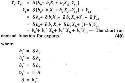
The short run partial derivative of Yt with respect to X1t is
δ Yt / δ X1t = b1*
The short run partial derivative of Yt with respect to X2t is
∂ Yt / ∂ X2t = b2*
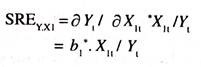
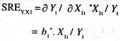
The short run partial elasticity of demand for exports with respect to world real income is
The long-run elasticity of demand for exports with respect to world real income is obtained by deflating the short-run elasticity as shown below:
LRE = b1*Xt/Yt* 1/δ
The short run partial elasticity of demand for exports with respect to relative price is
The long-run elasticity of demand for exports with respect to relative price is obtained by deflating the short-run elasticity with δ as shown below:
LRE = b2*X2t/Yt* 1/δ
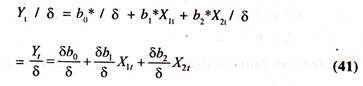
The long-run demand function for exports is obtained by deflating the short-run demand function for exports [obtained through the partial adjustment mechanism] with δ and deleting Yt-1 as shown below:
If the linear relationship between Yt and X1t and X2t is suitable to the data points then the other forms of equations have to be tried for estimating the short-run and long-run income and price elasticities. In empirical studies, the power function [log linear] is widely used.
The specification of the function will be as follows:
Yt* = b0 X1b1 X2b2
Y1* is desired level/equilibrium/long-run demand for exports which is un-observable.
Therefore, this function will be estimated with the following transformation using Nerlovians Partial Adjustment method:
logYt*= log b0+ b1 log X1t + b2 log X2t] [Long run demand function]………………. (42)
Yt.Yt-1 = [Yt* – Yt-1]δ
= logYt –logyt-1 ,= δ [log Yt*-log Yt-1] [Partia adjustment mechanism]………………. (43)
By substituting the long-run demand function for exports in the partial adjustment equation we get the following equation:
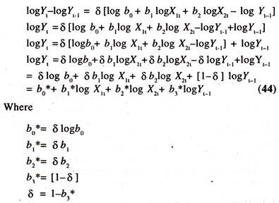
The above equation is known as the short-run demand function for exports.
The short-run demand function will be used for estimating the long-run demand function for exports with the help of coefficient of adjustment.
The short-run elasticity of demand for exports with respect to real world income will be obtained as follows:
∂ log Yt/∂ log X1t = b1*, whose value is would be positive.
The elasticity of demand for exports with respect to relative price will be obtained as follows:
∂ logYt/∂ log X2t = b2*, whose value will be negative.
The long-run elasticities of demand for exports with respect to income and prices will also be obtained by deflating the short-run elasticities as follows:
(i) The short run elasticity of demand for exports with respect to income/the coefficient of adjustment mechanism [δ].
LRE = ∂ log Yt/ ∂ log X1t / δ = b1*/δ
(ii) The short-run elasticity of demand for exports with respect to relative price/the coefficient of adjustment mechanism.
LRE = ∂ log Yt/ δ log X2t / δ = b2* / δ
The long-run elasticities will be relatively higher than the short- run elasticities. Thus, the partial adjustment model would be used for estimating the long-run and short-run demand functions for exports.
The coefficient of adjustment explains about the speed of adjustment between the desired change in demand for exports and actual change in demand for exports. If the value of coefficient of adjustment is close to one, then the speed of adjustment between the actual change and desired change in demand for exports will be very quick.
Demand Function for Exports and Interaction Variable:
The shift/structural change in the elasticity of exports with respect to world real income and relative price can be scanned by introducing an interaction variable [dummy variable X1t and dummy variable* X2t].
The specification of such function, log-linear form, will be as follows:
log Yt = log b0+ b1 log X1t+ b2[D * log xt] + b3 log X2t + b4 [D * log X2t) + error………….. (45)
The derivative of logYt with respect to IogX1t is b1, whose numerical value is known as the partial elasticity of Yt with respect to X1t in first period.(D = 0)
![]()
The value of differential elasticity of demand for exports with respect to world real income in the second period is b2. The sum of b1 + b2 is the partial elasticity of Yt with respect to X1t in the second period. (D = 1)
![]()
The derivative of log Yt with respect to log X2t is b3, whose numerical value is known as the partial elasticity of Yt with respect to X2t in first period.
![]()
The differential elasticity of Yt with respect to X2t in the second period is b4.
The derivative of log Yt with respect to log X2t is the sum of b3 + b4, known as the partial elasticity, in second period in second period.
![]()
If the time period is considered as period-I and period-II, the model in the period-I will be as follows; i.e., when D = 0 [Absence of attribute, for example, pre-economic reform period in India].
![]()
Specification of model in period-II i.e., when D = 1 [Presence of attribute for example post-economic reform period in India] will be as follows:
![]()
If b2 and b4 are statistically not significant, then the regression coefficient in period-I will be continued in period-II showing the stability. The advantage of fitting the double-log equation to the time series data with the interaction variable [dummy times, price variable or income variable] is that the problem of auto correlation can, to some extent, be reduced as compared to the results of the model fitted to the data without interaction variable.
Further, by fitting the single equation to the data, the two equations for period-I and period-II respectively can be obtained. In empirical studies, the double log equation is preferred to other equations on the grounds that the price and income elasticities of demand for exports will be directly obtained.
Apart from the price and income variables the other variables can also be considered for estimating demand function for exports [linear and log-linear demand functions] using OLS method. The inclusion of additional variables enables us to find the impact on the demand for exports.
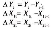
However the inclusion of additional variables in the function creates the problem of multi-collinearity, due to which the reliability of estimates would be in a weak position. Further the use of time series data creates the problem of auto-correlation due to which the precision of the estimates of the economic relationships would be suspected. This can to some extent be reduced by adopting the first differenced variables.
It should however be noted that, the OLS method is based on the assumption that time series data is stationary. If this assumption is not satisfied, then there will be a problem of unit root i.e., random walk. The presence of unit root in time series variable leads to spurious regression results.
The presence of unit root or non-stationarity in the time series variable can be detected by Augmented Dicky-Fuller [ADF] test. Most of the macro time the series data contains the problem of unit-root. Therefore, it has to be detected and the series needs to be corrected till stationarity is achieved.
As this is problem of a complicated one, most empirical works are carried out without testing the presence of unit root in the macro-time series variables. With the advent of software packages on econometrics, the presence of unit root [non- stationarity] can easily be detected.
Demand Function for Exports: Estimates of Economic Relationships:
The following results that emerged out of the empirical study explain the nature of elasticities of demand for exports with respect to world real income [X1] and export price [X2] [calculated from the linear demand function for Indian exports] for the period 1953 to 1962.

The average elasticity [estimated at mean values] of demand for exports with respect to export price was found to be -0.48 and with respect to world real income +0.20 explaining the inelastic nature of the Indian exports with respect to the price and income during the period 1953 to 1962.The 100 standard errors were found to be low, thus explaining that the two variables – price and real income were significantly influencing the exports.
The following results emerged out of the empirical study estimated by fitting the following log linear regression model by OLS method show the size and sign of the price and income elasticities of demand for exports for India and other selected countries for the period 1951-1966.
log Y = logb0 + b1logX1 – b2logX2
Where
Y = World demand for a given country’s aggregate exports
X1 = Real world income
X2 = Ratio of Unit value of exports to Export price index of the other country [This reflects the competition among the different suppliers to a given country]


The above results show that the income elasticities are significant [as the ‘t’ values within brackets are relatively higher because the standard errors are less than half of the regression coefficients: SE (bi) < bi/2] in all the countries under consideration but they are more than unity in Portugal Canada, West Germany and Japan evincing the elastic nature of the commodities exported. The price elasticities are significant only in Brazil and Canada.
The results of the demand function for Indian exports [commodity group of food, live animals and beverage and tobacco] for the period 1969-70 to 1989-90 show [table-5.3] that the signs of income and price elasticities are positive and negative respectively. They are less than unity showing the relatively inelastic nature of the commodities exported.
The following regression model was used:
log Y = log b0 + b1 log X1 + b2 logX2
Where
Y = Export quantity index
X1 = Ratio of unit value index of exports of a country to the unit value index of world exports
X2 = Index of world real income

Simple Demand Function for Exports:
In order to examine the responsiveness of gross exports [Y] to the changes in gross domestic product at current market prices [X] the linear [Y = b0 + b1X] and log linear [log Y = log b0 + b1 log X] regression models are fitted to nominal data [For the Indian Economy] given in table 5.4
Visual Plot:
The exports and income series move together in the same direction [Figure – 5[A]]


The regression results based on a simple linear demand function for exports in nominal terms are given in table 5.5

The regression results show that the regression coefficient of income is positively significant showing burly association between exports and income. The responsiveness of gross exports to the changes in income, based on average elasticity [ey.x] is 1.156, showing that the proportionate change in exports is relatively higher than the proportionate change in income.
In order to obtain constant elasticity of exports with respect to income a simple log linear demand function for exports is fitted to the data given in table 5.6.The results are given in table 5.7


The regression results based on a simple log linear demand function for Indian exports show that the coefficient of income, constant elasticity of exports with respect to income, is significantly positive. This explains that a one percent increase in income leads to increase the exports to 1.27 percent.
It should be noted that both in linear and log linear simple demand functions for exports the magnitude of the elasticity of Indian exports with respect to income is more than unity showing elastic nature of the Indian exports to the changes in income.