
The time value of money suggests a preference of having money as of now than at a future point of time.
The concept of time value of money helps in arriving at the comparable value of the different rupee amounts arising at different points of time into equivalent values at a particular point of time (present or future).
Learn about the techniques of time value of money: 1. Compounding Technique 2. Discounting or Present Value Technique
1. The compounding technique is used to find out the future value of different cash flows occurring at different points of time. According to this technique, interest earned on the initial principal or cash outflow becomes part of the principal for calculating interest for the next period. As a result interest is earned on interest as well as on the initial principal. This interest earned on interest is known as compounding effect and hence compounding technique.
ADVERTISEMENTS:
2. Discounting technique is used to make cash flows occurring over different future periods comparable at the present time. In this technique present worth of future cash flows are calculated.
Techniques of Time Value of Money: Compounding and Discounting or Present Value Technique (With Formulas and Examples)
Techniques of Time Value of Money – Compounding Technique and Discounting Technique (With Effective Rate of Interest)
These techniques of time value of money are now being discussed in detail:
Technique # 1. Compounding Technique:
The compounding technique is used to find out the future value of different cash flows occurring at different points of time. According to this technique, interest earned on the initial principal or cash outflow becomes part of the principal for calculating interest for the next period.
As a result interest is earned on interest as well as on the initial principal. This interest earned on interest is known as compounding effect and hence compounding technique.
ADVERTISEMENTS:
This compounding technique can be explained for calculating:
a. The future value of a single present cash flow.
b. The future value of a series of unequal cash flows over a period of time.
c. The future value of a series of equal cash flows over a period of time.
ADVERTISEMENTS:
d. The future value of a cash flow when compounding is done more than once in a year.
e. The future value of an annuity due.
a. The future value of a single present cash flow:
The mathematical formula of calculating compounding interest can be used in calculating the future value of a single present cash flow.
b. The future value of a series of unequal cash flows over a period of time:
When an investor has invested his money in unequal installments over a period of time, he may want to know the value of his investments after a certain period.
c. The future value of a series of equal cash flows over a period of time (FV of an annuity):
Let us take an example to understand the concept of an annuity. Mr. X has invested an equal amount say Rs. 10,000 each at the end of 1st, 2nd and 3rd year for 3 years at a certain rate of interest. This investment of equal amount or equal cash outflow can be termed as an annuity.
Another feature of an annuity is that cash flows (payment or receipt) should occur over a period of equal time intervals. Hence, an annuity can be defined as a series of equal cash flows (either inflows or outflows) occurring over a period of equal time intervals.
ADVERTISEMENTS:
We can find out the future value of an annuity by calculating the sum of future values of equal amount occurring over a period of equal time intervals as follows:
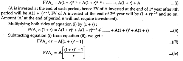
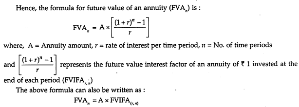
Assuming annuity amount as A, invested at the end of each period at r (rate of interest) over n periods of time, the formula for calculating future value of an annuity (FVAn) can be derived as follows –
FVIFA for different combinations of r and n can also be found from the future value interest factor of an annuity table.
d. The future value of a cash flow when compounding is done more than once in a year:
ADVERTISEMENTS:
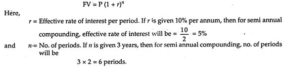
However, in many cases interest is compounded more than once in a year, say semi-annually, quarterly or even monthly. Formula for calculating the compounding value or FV of a cash flow when compounding is done more than once in a year will be same i.e. –
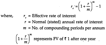
Concept of Effective and Stated (Normal) Rate of Interest:
Effective Rate of Interest:
The effective rate of interest is the rate of interest under annual compounding, which provides the same future value as provided by annual interest rate compounded more than once in a year.
ADVERTISEMENTS:
The concept of effective rate of interest is quite useful in financial decision making particularly in investment opportunities involving different compounding periods. Investment opportunity having the highest effective rate of interest is to be selected.
Mathematically, effective rate of interest and normal rate of interest (stated rate) are equal when they produce the same future value of an investment.
However, when compounding is done more than once in a year, the effective rate of interest will be higher than the stated annual rate of interest.
The relationship between the effective interest rate and the stated annual interest rate is as follows:
The following table shows the relationship between normal rate of interest of 12% per annum and effective rate of interest under different compounding periods:
Technique # 2. Discounting or Present Value Technique:
Discounting technique is used to make cash flows occurring over different future periods comparable at the present time. In this technique present worth of future cash flows are calculated.
ADVERTISEMENTS:
The present value approach works exactly in reverse of the compounding technique. In the case of compounding technique we ascertain the worth of all cash flows at a future date while in case of present value technique the worth of all future cash flows (both receipts or payments) are calculated at the present date by adjusting for time value of money.
We know money received in the future is less valuable than money received at present time. Therefore, the present value of future cash flow is calculated by multiplying it with a discounting factor. That is why this technique is known as a discounting technique.
Discounting technique can be explained for calculating:
a. Present value of a future sum.
b. Present value of a series of unequal cash flows.
c. Present value of a series of equal cash flows.
ADVERTISEMENTS:
a. Present Value of a Future Sum:
Present value of the money received in future will be less than the value of the same money in hand today. This is because the money in hand can be invested and its absolute value can be increased at a future date. Whereas money received in future has to be discounted to find its present value. Hence, discounting is the inverse of compounding.
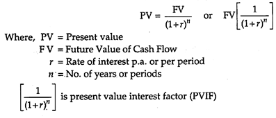
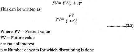
We can find the present value by restating the future value equation as follows:
b. Present Value of a Series of Unequal Cash Flows:
In most of the investment proposals, it is observed that unequal returns from these are spread over a number of years. For the title purpose of comparison, money received over future periods has to be discounted to present time and compared with initial investment.
The present value of a series of unequal cash flows can be calculated by using the following formula:
ADVERTISEMENTS:
DF1, DF2, DF3…. are the discounting factors (PVIF) for periods 1,2,3… taken from the table of PV of one rupee.
c. Present Value of a Series of Equal Cash Flows (Annuity):
However, when a business or individual gets constant cash inflows over a period of equal time intervals, such cash inflows are known as an annuity. We can find the present value of an annuity (PVA) by calculating the sum of present values of each equal cash inflow occurring over a period of equal time intervals.
Techniques of Time Value of Money – Compounding: Ascertaining the Future Value and Effective Rate of Interest
The time value of money suggests a preference of having money as of now than at a future point of time.
This implies that –
(a) a person will have to pay in future more for a rupee received today, implying thereby that the present value is compounded to arrive at future value;
ADVERTISEMENTS:
(b) A person may accept less today, for a rupee to be received in the future, implying thereby that the future value is discounted to arrive at present value. Therefore, the inverse of the compounding process is termed as discounting.
A series of cash flows may be compared with another series of cash flows either with reference to a future point of time or present date.
Accordingly, there are two valuation techniques to facilitate such comparison:
1. Compounding; and
2. Discounting.
1. Compounding Technique:
It is used to find out the future value of a given cash flow by ascertaining the compound interest for the period that is added to the principal (or initial) amount. The ascertainment of compound interest involves calculations for more than once a year, each using a new principal that is computed by adding interest to the principal.
The process of finding out the compound interest is based upon the principle of converting the interest into principal amount for the purpose of computing interest for the subsequent period. The period between two successive conversions of interest into the principal is called conversion period.
The number of conversion periods depends on how often the interest is calculated over the term of the investment (or loan) and must be determined for each year or fraction of a year.
For example, if the interest rate is compounded semi-annually, then there are two conversion periods per year. As a result, if the deposit (or loan) is for a period of five years, then the number of conversion periods would be ten.
If the interest rate is compounded quarterly, then the conversion periods are four and for a deposit (or loan) with a duration of five years, there would be 20 conversion periods.
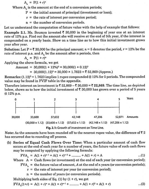
I. Ascertaining the Future Value (FV):
The compounding techniques that facilitate ascertainment of future value may be applied in the following specific situations:
(a) Single Cash Flow as at Present:
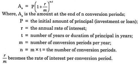
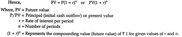
The future value of a single cash flow may be ascertained by applying the usual compound interest formula as given below:
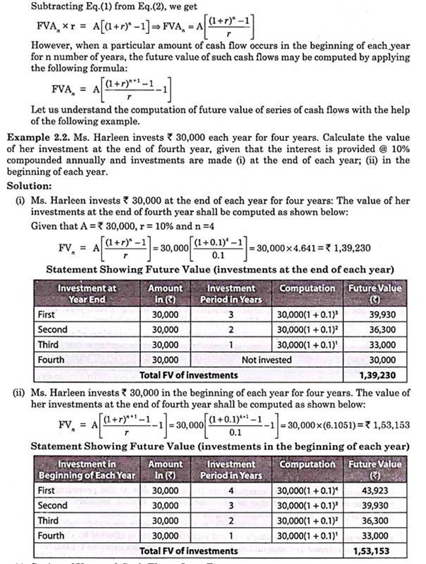
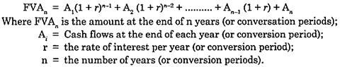
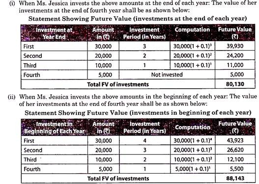
(c) Series of Unequal Cash Flows over Time:
When different amount of cash flow occurs in various years for a series of years, the future value of such cash flows may be computed by applying the following formula:
Let us understand the computation of future value of series of cash flows with the help of the following example.
Example:
Ms. Jessica invests Rs.30,000, Rs.20,000, Rs.10,000 and Rs.5,000 in first, second, third and fourth year respectively. Calculate the value of her investment at the end of fourth year, given that the interest is provided @ 10% compounded annually and investments are made
(i) at the end of each year;
(ii) at the beginning of each year.
Solution:
(d) Cash Flows with Multiple Compounding During the Year:
It is also known as discrete compounding. It is a method by which interest is computed and added to the principal amount after a certain point of time, and then the interest for every subsequent point of time is computed on the amount due at the preceding point in time. For example, interest may be compounded daily, weekly, monthly, quarterly or even half-yearly.
Discrete compounding is the opposite of continuous compounding, which uses a formula to compute interest as if it were being constantly calculated and added to principal. The investor’s annual yield (or return) is affected by the frequency with which interest is compounded.
For example, if a person deposits Rs.1,00,000 in an account to earn 5% interest annually, then on the basis of annual compounding, he will have at the end of the year Rs.1,05,000 while on the basis of monthly compounding and daily compounding, he will have Rs.1,05,116.19 and Rs.1,05,126.75 respectively.
The following formula is used for computing the compound interest, discreetly:
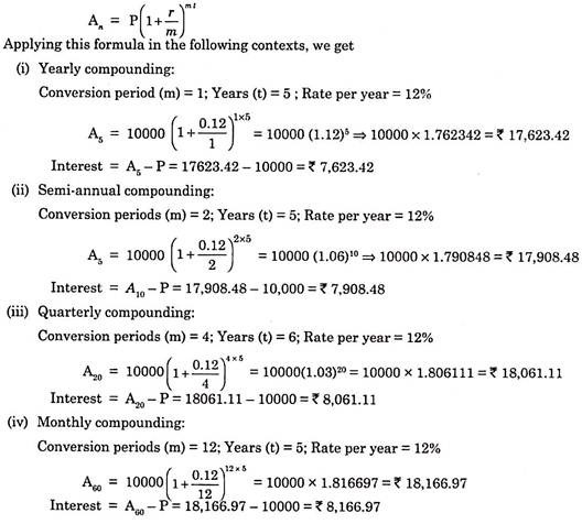
Example:
Ms. Soumya invested Rs.10,000 for five years at an interest rate of 12% p.a. Find out the interest on investment, if the interest is compounded (i) yearly, (ii) semi-annually, (iii) quarterly; and (iv) monthly.
Solution:
Let P be the principal amount; m denotes the conversion periods per year, t denotes number of years, r be the rate of interest p.a. and An be amount after n = mt conversion periods, then –
II. Ascertaining Effective Rate of Interest:
There are two types of interest rates:
(a) Nominal rate and
(b) Effective rate
that need to be understood from the perspective of borrower and lender.
(a) Nominal Rate:
The nominal interest rate, which is also known as an Annualized Percentage Rate (APR), is the periodic interest rate that is multiplied by the number of periods per year. For example, a monthly rate of 0.75% implies a nominal annual interest rate of 9% (i.e. 0.75% x 12). Likewise, a quarterly rate of 2.25% implies a nominal annual interest rate of 9% (i.e. 2.25% x 4).
But both the nominal interest rates, though identical, are not comparable because of their different compounding periods. In the context of inflation, a nominal rate implies a rate before adjusting for the impact of inflation. There is a Fisher equation that is used to convert nominal rate into real rate, which is inflation adjusted rate. However, current literature on financial studies uses APR rather than nominal rate to describe the difference between effective rate and APR’s.
(b) Effective Interest Rate:
Nominal interest rates are not comparable unless their compounding periods are the same. The effective interest rate makes a correction for this by transforming nominal rates into annual compound interest. The effective interest rate is computed by taking into account the effect of compounding during the year.
In many cases, interest rates, as quoted by lender, are based on nominal, not effective interest rates. As a result, the lender may understate the interest rate compared to the equivalent effective annual rate.
Relationship between Nominal Rate and Effective Rate:
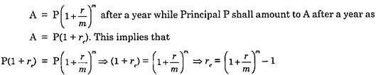
As the effective rate of interest is computed on the basis of nominal rate of interest, a definite mathematical relationship exists between nominal rate and effective rate of interest. Let us understand this relationship for discrete compounding.
Let r denote nominal rate of interest per annum and m as the number of conversion periods during a year, P as the principal amount and r, be the effective rate per annum, then the amount obtained by compounding P shall be:
Example:
Mr. Sudhanshu wishes to open a fixed deposit account with a bank. Each bank offers interest @ 10% p.a. However, Bank-A compounds annually; Bank-B semi-annually; Bank-C Quarterly; Bank-D Monthly and Bank-E Weekly. You are required to suggest the bank in which he should open his fixed deposit account.
Solution:
Let re denote effective rate; r denotes nominal rate, and m refers to conversion periods per year, then we have r = 10%, m = 1, 2, 4, 12 and 52 for Bank – A, B, C, D and E respectively.
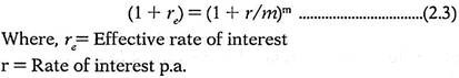
Applying the following formula for effective rate, we get re = (1+(r/m))m – 1
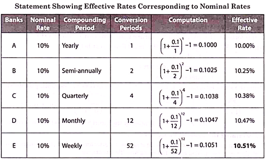
Since the highest effective rate is offered by Bank E, Mr. Sudhanshu should open his fixed deposit account with Bank E to get the effective rate of 10.51% p.a.
Techniques of Time Value of Money – Compounding Technique and Discounting Value Technique
The techniques of time value of money are as follows:
1. By compounding the various cash flows to a future date, or
2. By discounting the various cash flows to the present date.
These techniques of compounding and discounting are now being discussed in detail:
1. Compounding Technique:
The compounding technique is used to find out the future value of different cash flows occurring at different points of time. According to this technique, interest earned on the initial principal or cash outflow becomes part of the principal for calculating interest for the next period.
As a result interest is earned on interest as well as on the initial principal. This interest earned on interest is known as compounding effect and hence compounding technique.
This compounding technique can be explained for calculating:
a. The future value of a single present cash flow.
b. The future value of a series of unequal cash flows over a period of time.
c. The future value of a series of equal cash flows over a period of time.
d. The future value of a cash flow when compounding is done more than once in a year.
e. The future value of an annuity due.
a. The future value of a single present cash flow:
The mathematical formula of calculating compounding interest can be used in calculating the future value of a single present cash flow.
b. The future value of a series of unequal cash flows over a period of time:
When an investor has invested his money in unequal installments over a period of time, he may want to know the value of his investments after a certain period.
c. The future value of a series of equal cash flows over a period of time (FV of an annuity):
Let us take an example to understand the concept of an annuity. Mr. X has invested an equal amount say Rs. 10,000 each at the end of 1st, 2nd and 3rd year for 3 years at a certain rate of interest. This investment of equal amount or equal cash outflow can be termed as an annuity.
Another feature of an annuity is that cash flows (payment or receipt) should occur over a period of equal time intervals. Hence, an annuity can be defined as a series of equal cash flows (either inflows or outflows) occurring over a period of equal time intervals.
We can find out the future value of an annuity by calculating the sum of future values of equal amount occurring over a period of equal time intervals as follows:
Assuming annuity amount as A, invested at the end of each period at r (rate of interest) over n periods of time, the formula for calculating future value of an annuity (FVAn) can be derived as follows –
d. The future value of a cash flow when compounding is done more than once in a year:
However, in many cases interest is compounded more than once in a year, say semi-annually, quarterly or even monthly. Formula for calculating the compounding value or FV of a cash flow when compounding is done more than once in a year will be same i.e. –
Concept of Effective and Stated (Normal) Rate of Interest:
Effective Rate of Interest:
The effective rate of interest is the rate of interest under annual compounding, which provides the same future value as provided by the annual interest rate compounded more than once in a year.
The concept of effective rate of interest is quite useful in financial decision making particularly in investment opportunities involving different compounding periods. Investment opportunity having the highest effective rate of interest is to be selected.
Mathematically, effective rate of interest and normal rate of interest (stated rate) are equal when they produce the same future value of an investment.
However, when compounding is done more than once in a year, the effective rate of interest will be higher than the stated annual rate of interest.
The relationship between the effective interest rate and the stated annual interest rate is as follows:
The following table shows the relationship between normal rate of interest of 12% per annum and effective rate of interest under different compounding periods: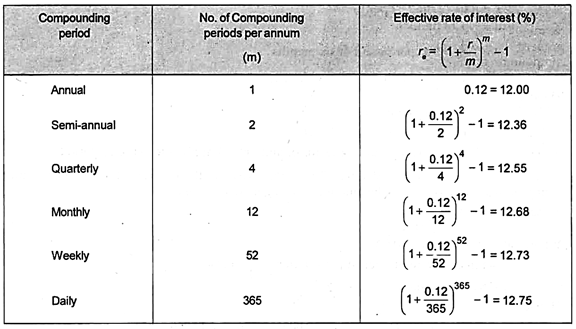
2. Discounting or Present Value Technique:
Discounting technique is used to make cash flows occurring over different future periods comparable at the present time. In this technique present worth of future cash flows are calculated.
The present value approach works exactly in reverse of the compounding technique. In the case of compounding technique we ascertain the worth of all cash flows at a future date while in case of present value technique the worth of all future cash flows (both receipts or payments) are calculated at the present date by adjusting for time value of money.
We know money received in the future is less valuable than money received at present time. Therefore, the present value of future cash flow is calculated by multiplying it with a discounting factor. That is why this technique is known as a discounting technique.
Discounting technique can be explained for calculating:
a. Present value of a future sum.
b. Present value of a series of unequal cash flows.
c. Present value of a series of equal cash flows.
a. Present Value of a Future Sum:
Present value of the money received in future will be less than the value of the same money in hand today. This is because the money in hand can be invested and its absolute value can be increased at a future date.
Whereas money received in future has to be discounted to find its present value. Hence, discounting is the inverse of compounding.
We can find the present value by restating the future value equation as follows:
b. Present Value of a Series of Unequal Cash Flows:
In most of the investment proposals, it is observed that unequal return from these are spread over a number of years. For the title purpose of comparison, money received over future periods has to be discounted to present time and compared with initial investment.
The present value of a series of unequal cash flows can be calculated by using the following formula:
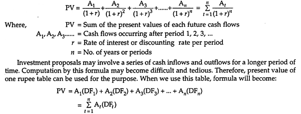
DF1, DF2, DF3…. are the discounting factors (PVIF) for periods 1,2,3… taken from the table of PV of one rupee.
c. Present Value of a Series of Equal Cash Flows (Annuity):
However, when a business or individual gets constant cash inflows over a period of equal time intervals, such cash inflows are known as an annuity. We can find the present value of an annuity (PVA) by calculating the sum of present values of each equal cash inflow occurring over a period of equal time intervals.
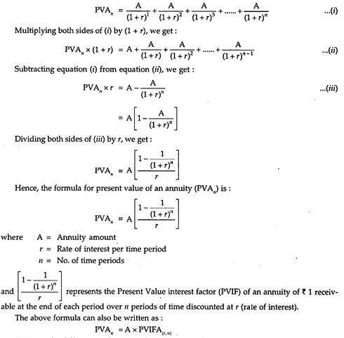
Assuming annuity amount as A, receivable at the end of each period, over n period of time and discounted at r (rate of interest), the formula for calculating the present value of an annuity (PVAn) can be derived as follows –
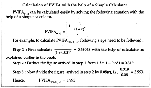
PVIFA(r,n) for different combinations of r and n can be found out from the present value interest factor of an annuity table.
Techniques of Incorporating Time Value of Money – Compounding and Discounting Technique (With Examples and Solutions)
There are two techniques of incorporating Time value of money concept into financial decision making.
They are explained in detail below:
Technique # I. Compounding:
The compounding technique helps in finding out the future value of current or present amount of money.
It can be explained under the following two heads:
A. Future Value of a Lump Sum Amount (Single Sum of Money):
(i) In Case of Annual Compounding:
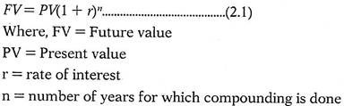
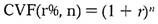
The future value of present money can also be found out by multiplying the present value by a Compound Value Factor (CVF). Compound value factor is nothing but the value of (1 + r)n for a given rate of interest (r) and number of years (n). By looking at the Table of CVF (r%, n) you can see that one can obtain compound value factor for several combinations of r and n.
Please note that:
Compound Value Factor for a Lump Sum Amount (CVF) (r%, n) you find that the cell value where r= 15% and n=5 years is 2.011. It implies that Re 1 received today has a future value of Rs.2.011 at the end of 5 years if the rate of interest is 15%.
Hence to calculate future value we can also use the following formula:

Example:
Mr. X deposits Rs.100000 on 1st January 2015 in a Bank at 12% rate of interest compounded annually for two years. Find out the Future value of the deposit as on 31st Dec 2016.
Solution:
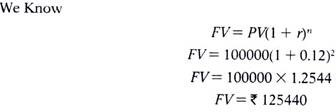
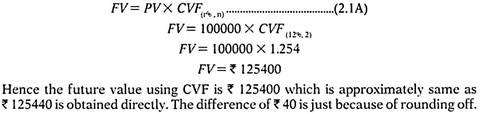
The future value of present money can also be found out by multiplying the present value by a Compound Value Factor (CVF).
So, in the above example, Future value can also be calculated as:
(ii) In Case of Non-Annual Compounding:
It is quite possible that interest is not compounded annually but at a lesser interval say semiannually, quarterly or even monthly. Please note that nowadays banks provide interest on a daily compounding basis.
If interest is compounded semiannually or every six months then in a year we have two compounding. In this case if the numbers of years are 5 then the number of compounding will be 10 (5 X 2). This requires some adjustment in the formula given in equation (2.1). We divide by the number of compounds in a year (m) and at the same time multiply n by the number of compounds in a year (m).
Please note that in case of semiannual compounding (i.e. compounding every six month) the value of m will be 2 because there are 2 compounds in a year. When compounding is done on a quarterly basis (every 3 month) then the value of m will be 4. When the compounding is done on a monthly basis then the value of m will be 12 because then there are 12 compounds in a year.
If the time period ‘n’ is not annual, then the formula for calculating the future value will be modified as follows:
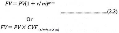
Where, m = number of times of compounding per year. We need to divide r by m and multiply n by m so as to calculate future value of a present sum of money.
Example:
Find out the future value in Example if the rate of interest is compounded quarterly.
Solution:
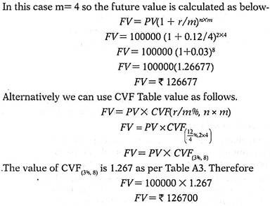
This value is similar to the one that we obtained without using Table values i.e. 126677. Please note that the difference of Rs.23 is just because of rounding off of the Table values.
We can observe that future value is higher when compounding is done quarterly rather than annually. Thus, more frequently the compounding is made; the higher will be the future value.
(iii) Rate of Interest p.a. vs. Effective Annualised Rate of Interest:
Rate of interest p.a. assumes that interest is compounded annually. However, if interest is not compounded on an annual basis but on the basis of semiannual, quarterly etc., then we need to consider the effective annualised rate of interest. This is because in such a case the effective annualised rate of interest will be higher due to more frequent compounding.
Therefore there is no difference between Rate of interest p.a. and Effective annualised rate of interest if the compounding is done annually. This is because in that case there is one compounding every year which is also assumed by Rate of interest p.a.
However, if there is ‘m’ times compounding every year, the effective annualised rate of interest can be calculated as:
Example:
Find out the effective annualised rate of interest if rate of interest is 12% p.a. and compounding is done on quarterly basis.
Solution:
In this case compounding is done on quarterly basis hence Effective rate can be calculated as:
It implies that if the interest is compounded on quarterly basis, 12% p.a. interest provides an effective annualised rate of interest of 12.55%.
It shows that the more frequent compounding generates higher effective annualised rate of interest.
This is the reason why investors prefer more frequent compounding for their invested money.
B. Future Value of an Annuity (i.e. a Series of Equal Cash Flows):
A series of equal cash flows occurring every year (at the end of the year) for a number of years continuously is called an Annuity.
Assume that you receive Rs.1000 at the end of every year for each of the next five years. Then in total you receive Rs.5000 over a 5 years period. But in finance we cannot say that the value of Rs.1000 received every year for 5 years is Rs.5000. This is because these amounts occur at different points of time. First amount of Rs.1000, at the end of first year, second amount of Rs.1000 at the end of second year and so on.
In order to calculate Future value of this series of Rs.1000 cash every year for 5 years we can proceed as follows:
The first Rs.1000 which is received at the end of first year will be compounded for 4 years to find its value at the end of 5th year. This is because Rs.1000 is not received now but at the end of 1st year which is nothing but the beginning of second year.
So it can be invested in the beginning of 2nd year to earn interest on it. Till the end of 5th year it would have been staying invested for 4 years i.e. for 2nd, 3rd, 4th and 5th year. Hence this Rs.1000 will earn interest for 4 years.
The second Rs.1000 which is received at the end of 2nd year will be compounded for 3 years to find its value at the end of 5th year. This is because Rs.1000 is not received now but at the end of 2nd year which is nothing but the beginning of 3rd year.
So it can be invested in the beginning of 3rd year to earn interest on it. Till the end of 5th year it would have been staying invested for 3 years i.e. for 3rd, 4th and 5th year. Hence this Rs.1000 will earn interest for 3 years.
The third Rs.1000 which is received at the end of 3rd year will be compounded for 2 years to find its value at the end of 5th year. This is because Rs.1000 is not received now but at the end of 3rd year which is nothing but the beginning of 4th year.
So it can be invested in the beginning of 4th year to earn interest on it. At the end of 5th year it would have been staying invested for 2 years i.e. for 4th and 5th year. Hence this Rs.1000 will earn interest for 2 years.
The fourth Rs.1000 which is received at the end of 4th year will be compounded for 1 years to find its value at the end of 5th year. This is because Rs.1000 is not received now but at the end of 4th year which is nothing but the beginning of 5th year.
So it can be invested in the beginning of 5th year to earn interest on it. At the end of 5th year it would have been staying invested for 2 year i.e. for 5th year. Hence this Rs.1000 will earn interest only for 1 year.
The last Rs.1000 which is received at the end of 5th year does not need any compounding because it is already at the end of 5th year.
Therefore Future Value of this Annuity of Rs.1000 can be calculated as follows:
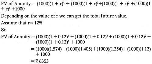
Thus Rs.1000 received at the end of every year for 5 years at 12% rate of interest will be Rs.6353 at the end of 5th year.
Hence the future value of the annuity of Rs.1000 in our example is Rs.6353.
Short Method – Using Compound Value Annuity Factor Table:
We can calculate the series of these cash flows by using CVAF (r%, n) Compound Value Annuity Factor for r% and n years.
The generalised formula for calculating future value of an annuity is given below:
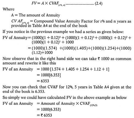
It must be noted that CVAF (12%, 5) of 6.353 is the compound value or future value of Re 1 invested at the end of every year for 5 years at 12% interest rate p.a.
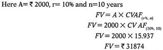
Example :
Mr. Raja opens a recurring account in a Bank where he deposits Rs.2000 every year for 10 years at 10% p.a. What is the future value of his amounts deposited in the Bank.
Solution:
Mr. Raja is depositing Rs.2000 every year for 10 years. Hence this is the case of an Annuity. The future value of his annuity can be found out by multiplying the annuity amount by compound value annuity factor that can be obtained from “Compound Value Annuity Factor Table” (CVAF Table).
Technique # II. Discounting Technique:
In the case of compounding technique we calculated the value of the money in future points of time.
In the case of the Discounting technique we calculate the value of the money in the present point of time.
Thus the discounting technique helps in finding out the present value of money to be received in future. It is the reverse of compounding technique which helps in finding out the future value of present money.
It can be explained under the following two heads:
(i) Present Value of a Lump Sum Amount (a Single Sum of Money):
We know from equation (2.1) that:
Please note that Present value of a series of unequal cash flows is simply the sum total of the present value of each of the cash flows.
Example:
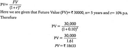
Mr. A is to receive Rs.30,000 at the end of 5 years from now. If the interest rate is 10% p.a., find out the present value of Rs.30000.
Solution:
Present value formula is:
The present value of a future sum can also be found out by multiplying the future value by a present value factor that can be obtained from “Present Value of a Given Amount Table”. From the PVF Table, one can obtain a present value factor for several combinations of r and n.
So we can have:
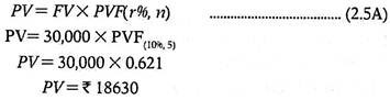
Please note that this is the same as calculated without using Table values. The minor difference of Rs.3 is due to rounding of.
(iii) Present Value of a Perpetuity:
An Annuity is a series of equal cash flows occurring at regular intervals for a finite or defined period of time.
Perpetuity consists of an infinite series of equal cash flows occurring at regular intervals for an indefinite period of time.
The present value of such perpetuity can be calculated as follows:
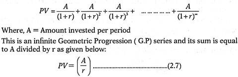
Example:
Mr. A invests Rs.20000 every year indefinitely in a recurring bank deposit account, which earns him 5% p.a. Find out the Present value of such perpetuity.
Solution: 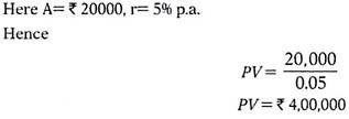
Annuity Due:
Annuity due is different from ordinary Annuity in the sense that under annuity due, the cash flows occur in the beginning of each period instead of occurring at the end of each period.
Please note that in case of an Annuity, the same amount of cash flows occur at the end of every year. In case of an Annuity Due, the same amount of cash flows occur in the beginning of every year.
Therefore in case of compounding an Annuity due will have one more year for compounding in case of each cash flow. Therefore while calculating Future value of an Annuity Due we multiply the Future Value of an Annuity by (1 + r) so as to increase the compound value factor by one year.
However in case of discounting, i.e. while calculating Present value of an Annuity Due, we have one year less for discounting because cash flows occur in the beginning of every year rather than at the end. Therefore while calculating the Present value of an Annuity Due we multiply the Present Value of an Annuity by (1 + r) so as to reduce the present value factor by one year.
(i) Future Value of Annuity Due:
In case of compounding an Annuity due will have one more year for compounding in case of each cash flow. Therefore while calculating the Future value of an Annuity Due we multiply the Future Value of an Annuity by (1+r) so as to increase the compound value factor by one year.
Future value of an Annuity Due can be calculated as below: 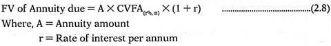
Example:
Mr. Anuj deposits Rs.40000 in the beginning of every year for 10 years at the rate 8% p.a. How much will he get after the expiry of 10 years?
Solution:
Since an equal amount is deposited in the beginning of every year, this is the case of an Annuity Due. Here we are given that A = Rs.40000, n= 10 years and r = 8% p.a.
Therefore,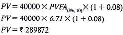
Hence Mr. Anuj will get Rs.625838 at the end of 10th year,
(ii) Present Value of Annuity Due:
In case of discounting, i.e. while calculating Present value of an Annuity Due, we have one year less for discounting because cash flows occur in the beginning of every year rather than at the end. Therefore while calculating the Present value of an Annuity Due we multiply the Present Value of an Annuity by (1 + r) so as to reduce the present value factor by one year.
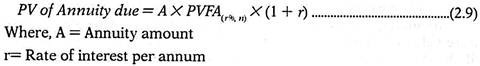
Present value of an Annuity Due can be calculated as below:
Example:
Anu deposits Rs.40000 in the beginning of every year for 10 years at the rate 896 p.a. What is the present value of total deposits made by Anu?
Solution:
Since an equal amount is deposited in the beginning of every year, this is the case of an Annuity Due. Here we are given that A = Rs.40,000, n = 10 years and r = 8% p.a.
Therefore,
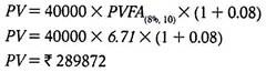
Therefore, we can say that the present value of all the deposits made by Anu is Rs.289872.
Techniques of Time Value of Money – Compounding and Discounting (With Formulas)
The methods for dealing with time value of money are:
The concept of time value of money helps in arriving at the comparable value of the different rupee amounts arising at different points of time into equivalent values at a particular point of time (present or future).
The techniques of time value of money are as follows:
(i) Compounding (or)
(ii) Discounting
Technique # (i) Compounding
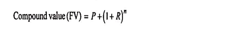
The concept of compounding refers to ascertainment of future value of present money. It is the same as the concept of compound interest, wherein the interest earned in the preceding year is reinvested at the prevailing rate of interest for the remaining period.
Thus, the accumulated amount (Principal + interest) at the end of a period becomes the principal amount for calculating the interest for the next period.
The compounding technique to find out the future value (FV) of a present money is discussed under the following heads:
(a) Compounding of interest over ‘n’ years:
The interests of investment are generally spread over a number of years. These interests are to be compounded annually to ascertain the future value/maturity value of investment.
The compounding of interest can be done with the help of the following formula:
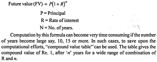
(b) Multiple compounding periods:
It is presumed that the time period “n” is an annual period and the compounding is done on an annual basis only. However, the compounding period ‘n’ may be other than a year also. In such a case, the compounding formula is to be adjusted to reflect different numbers of periods.
For example, if the compounding is done every 6 months, then the time period ‘n’ will become 2 times in a single year. Similarly, the interest rate is also to be adjusted, because the rate of interest will remain the same, but the interest amount of any 6 month will be compounded in the next 6 month and so on.
The more frequently the interest is compounded, the faster a future value (FV) grows. Further, more frequently the interest is compounded, it begins in turn to earn further interest and hence higher in the effective annual compound rate of interest.
In this case, the following formula is generally applied to ascertain the compound value:
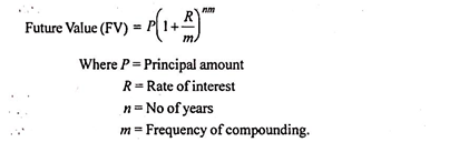
In the case of multiple compounding periods also, the compound value can be found by using “compound value table”. But the procedure is slightly different. Compound value is to be located for (n x m) years at (R/m) interest.
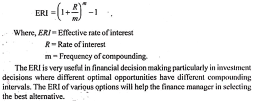
(c) Effective rate of interest:
The effective rate of interest is the annually compounded rate of interest that is equivalent to an annual interest rate compounded more than once per year. The effective rate of interest and the nominal rate of interest are equal whenever they generate the same future value (FV).
The effective rate of interest can be ascertained by applying the formula given below:
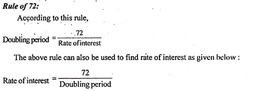
(d) Doubling period:
Sometimes, investors and financial decision makers are interested in knowing the time required for doubling their investment amounts. Such a period is called the ‘doubling period’. When interest rates ruled high in the nineties, investment made in Indira Vikas Patra was doubled in 5 years. An investment of Rs. 1,00,000 became Rs. 2,00,000 in 5 years. Rule of thumb methods known as rule of 72 and rule of 69 can be applied to ascertain the doubling period.
Rule of 69:
Rule of 69 is a refinement over rule of 72. It provides a more accurate result.
The formula is:

(e) Compound value of a series of payments:
In case payments are made at different points of time, such as at the end of first year, second year, third year, fourth year and so on, the compound value is received only after the specified period, say 4 years. In such cases, the first payment remains locked up for 3 years (n – 1), second payment remains locked up for 2 years (n – 2) and so on.
The formula for calculation of compound value in this case is as follows:
Instead of using the above formula, the compound value can also be ascertained by using ‘compound value table’.
(f) Compound value of an annuity:
Quite often a decision may result in the occurrence of cash flows of the same amount every year for a number of years consecutively, instead of a single cash flow. For example, a deposit of Rs. 5,000 each year is to be made at the end of each of the next 3 years from today.
This may be referred to as an annuity of deposit of Rs. 5,000 for 3 years. An Annuity is thus, a finite series of equal cash flows made at regular intervals. In the case of annuity, each cash flow is to be compounded to ascertain its FV. The total of these FVs of all these cash flows will be the total FV of the annuity.
The FV of annuity can be ascertained by using the formula given below:
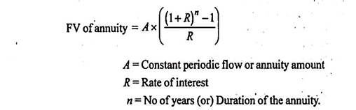
From the above formula, it is clear that the FV of annuity is dependent upon three variables i.e., the annual amount, the rate of interest and the time period. If any of these variables changes, it will change the future value of the annuity.
The future value of the annuity can also be ascertained by using a table showing compounding factor of an annuity. In this table, the value given at the intersection of a particular rate of interest and particular number of years, when multiplied by the amount of annuity gives the future value (FV) of the annuity.
Technique # (ii) Discounting or Present value technique
After having gone through the process of determining the future value (FV) of a present money or a present series, now the process of finding out the present value (FV) of a future sum or a future series can be discussed.
This process is in fact the reverse of compounding technique and is known as the discounting technique (or) present value technique. As there are future values (FVs) of sums invested now, calculated as per the compounding techniques, there are also the present values of a cash flow scheduled to occur in future.
The ascertainment of present value of future cash flows under discounting technique is discussed under the following heads:
(a) Present value of a lump sum:
The present value of a future sum will be worth less than the future sum because one forgoes the opportunity to invest and thus foregoes the opportunity to earn interest during that period.
Expectations of receiving money in future means that the money is not available presently and therefore one has to forego the interest which could be earned, had the money been available now. This also makes a person lose the opportunities to get return in terms of interest earnings on that investment.
This interest foregone is the cost to the investor and the future expected money must be adjusted for this cost. As the length of time for which one has to wait for the future money increases, the cost attached to delay also increases reflecting the compounded value of the lost opportunities.
In order to find out the PV of the future money, this opportunity cost of the money is to be deducted from the future money.
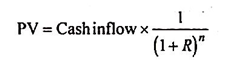
Say, Rs.2,200 is receivable at the end of one year from now and the expected rate of interest which a person can earn on his investment is 10% p.a, then the present value (PV) can be calculated with the help of the following formula:
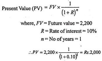
This means that Rs.2,200 receivable after 1 year is just equal in worth of Rs. 2,000 receivable today. The formula for calculation PV given above indicates that PV of a future money depends upon the three variables i.e. the future value, the rate of interest and the time period. Instead of ascertaining the PV through the above mentioned formula, the same can be found out by referring to PV table.
The figure given at the intersection of a particular rate of interest, R and time period ‘n’, when multiplied by the future value will give the PV of that amount for the given combination of ‘R’ and ‘n’.
The formula for calculation of PV through PV table can be written as follows:
PV = FV x PVF
For example, in order to find out the PV of Rs. 10,000 receivable after 4 years and the rate of interest at 12%, the PV factor in the PV table (12% column and 4 years row) is 0.635. Now Rs. 10,000 x 0.635 = Rs. 6,350 is the PV of Rs. 10,000. It means that an amount of Rs. 6,350 invested at 12% p.a for 4 years will accumulate to Rs. 10,000.
Thus, the PV of future money is the amount that makes a person exactly as well off today as the money received in future.
Two things can be observed in the value given in the PV table i.e:
(i) for a given period, the higher the interest rate, the lower will be the present value factor and therefore, the lower will be the PV, and
(ii) for a given rate of interest, the longer the time period, the lesser will be the present value factor and therefore, the lower will be the PV.
The reason for this behaviour is quite clear. As the length of waiting time to receive the future money increases, the PV factor also decreases reflecting the continuation of the lost opportunities to earn interest for a longer period.
(b) Present value of a series of cash flows:
The returns on investment are generally spread over a number of years. The investment made now may yield returns for a period after sometime. The investor is normally interested in knowing whether it is worth to invest or forego a certain sum now, in anticipation of returns he will earn over a number of years.
To take decision on this, he will have to equate the total anticipated future returns, to the present sum he is going to sacrifice. To determine the present value of future series of cash flows, the PV of different cash flows accruing at different times is to be calculated and then added.
The PV of different cash flows can be ascertained by using the following formula:
Instead of using the above mentioned formula, the P.V. of different cash flows can also be found out by using P.V. table.
(c) Present value of an annuity:
In the above case, the cash flows may be of different amounts. But in certain cases, the investor may receive only constant returns over a number of years. For example, interest on debentures/fixed deposits etc. is fixed in its nature. Such fixed return is termed as annuity.
To ascertain the PV of annuity, the formula given below may be used:

The above formula indicates that the P.V. of annuity also depends upon three variables i.e. the annuity amount, the rate of interest and the time period. Instead of applying the above said formula, the P.V. of annuity can also be determined by referring to P.V. of the annuity table.
In this table, any combination of ‘R’ and ‘n’ will give a value which, if multipxlied by the annuity amount, will give the P.V. of the annuity for that particular rate of interest and time period.
(d) Present value of annuity due:
The P.V. of annuity discussed is based on the presumption that the cash flows occur at the end of each of the periods starting from now. However in practice, the cash flow may also occur in the beginning of each period. Such a situation is called annuity due.
The present value of annuity due can be found out by applying the following formula:
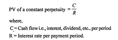
(e) Present value of a perpetuity:
Perpetuity is a stream of payments or a type of annuity that starts payments on a fixed date and such payments continue forever i.e., perpetually. Thus, perpetuity is a constant stream of identical cash flows with no end.
Examples of perpetuity are:
(i) Dividend on irredeemable preference share capital;
(ii) Interest on irredeemable debt/bonds and
(iii) Scholarships paid perpetually from an endowment fund etc.
The present value of perpetuity can be ascertained by using the following formula:
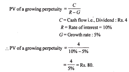
(f) Present value of growing perpetuity:
A growing perpetuity is an infinite series of periodic cash flows which grow at a constant rate per period.
The P. V. of growing perpetuity can be determined by applying the following formula:
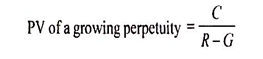
where,
C = cash flow i.e., interest, dividend per period
R = Interest rate per payment period
G = Rate of growth in cash flows
However, it may be noted that the above formula can be used only if the rate of interest is more than the rate of growth (R > G). For example, a company is expected to declare a dividend of Rs. 4 at the end of first year from now and this dividend is expected to grow 5% every year.
What is the PV of this stream of dividend if the rate of interest is 10%? The PV for this dividend stream is calculated as given below:
(g) Present value of a growing annuity:
A growing annuity is a finite series of equal and periodic cash flows growing at a constant rate every period. Let us take an example to make this concept clearer. Mr. Rama engages in a part time job for 5 years to finance for his studies in an evening college.
His employer fixes an annual salary of Rs. 24,000 with the provision that he will get an annual increment of 10. It means that he will get the following amounts from year 1 through year 5.
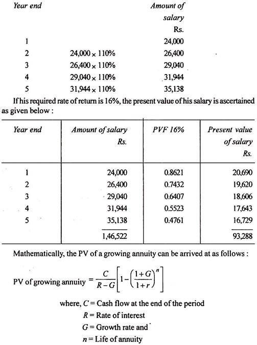
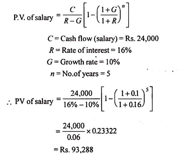
The present value of salary, for the example given above, can also be ascertained by using mathematical formula:
(h) Sinking fund:
It is a fund created by investing a certain amount annually at compound interest for a certain period, at the end of which such accumulated funds are used to discharge a known liability (or debentures) or to replace a working asset.
In this case, the annual accumulation becomes the annuity for a given period where each of the annual accumulations will be invested for the remaining period so that the total accumulation at the end of the given period is equal to the target amount.
For example, an amount of Rs. 2,00,000 is required at the end of 5 years from now to repay a debentures liability. What amount should be accumulated every year at a 12% rate of interest so that it ultimately becomes Rs. 2,00,000 after 5 years?
The annual accumulation (installment) can be arrived at by applying the formula given below:
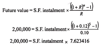
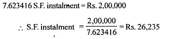
Therefore, an amount of Rs. 26,235 should be accumulated and invested at 12% rate of interest. This will accumulate to a total of Rs. 2,00,000 by the end of 5 years.
The above calculation was made on the presumption that annual S.F. installment payment occurs at the end of each of the periods starting from now. However, in practice, the annual S.F. installment payment may also occur at the beginning of each period.
In such situation, the annual accumulation (installment) is to be arrived at by using the formula given below: 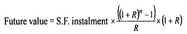
The time value of money suggests a preference of having money as of now than at a future point of time.
The concept of time value of money helps in arriving at the comparable value of the different rupee amounts arising at different points of time into equivalent values at a particular point of time (present or future).
Learn about the techniques of time value of money: 1. Compounding Technique 2. Discounting or Present Value Technique
1. The compounding technique is used to find out the future value of different cash flows occurring at different points of time. According to this technique, interest earned on the initial principal or cash outflow becomes part of the principal for calculating interest for the next period. As a result interest is earned on interest as well as on the initial principal. This interest earned on interest is known as compounding effect and hence compounding technique.
2. Discounting technique is used to make cash flows occurring over different future periods comparable at the present time. In this technique present worth of future cash flows are calculated.
Techniques of Time Value of Money: Compounding and Discounting or Present Value Technique (With Formulas and Examples)
Techniques of Time Value of Money – Compounding Technique and Discounting Technique (With Effective Rate of Interest)
These techniques of time value of money are now being discussed in detail:
Technique # 1. Compounding Technique:
The compounding technique is used to find out the future value of different cash flows occurring at different points of time. According to this technique, interest earned on the initial principal or cash outflow becomes part of the principal for calculating interest for the next period.
As a result interest is earned on interest as well as on the initial principal. This interest earned on interest is known as compounding effect and hence compounding technique.
This compounding technique can be explained for calculating:
a. The future value of a single present cash flow.
b. The future value of a series of unequal cash flows over a period of time.
c. The future value of a series of equal cash flows over a period of time.
d. The future value of a cash flow when compounding is done more than once in a year.
e. The future value of an annuity due.
a. The future value of a single present cash flow:
The mathematical formula of calculating compounding interest can be used in calculating the future value of a single present cash flow.
b. The future value of a series of unequal cash flows over a period of time:
When an investor has invested his money in unequal installments over a period of time, he may want to know the value of his investments after a certain period.
c. The future value of a series of equal cash flows over a period of time (FV of an annuity):
Let us take an example to understand the concept of an annuity. Mr. X has invested an equal amount say Rs. 10,000 each at the end of 1st, 2nd and 3rd year for 3 years at a certain rate of interest. This investment of equal amount or equal cash outflow can be termed as an annuity.
Another feature of an annuity is that cash flows (payment or receipt) should occur over a period of equal time intervals. Hence, an annuity can be defined as a series of equal cash flows (either inflows or outflows) occurring over a period of equal time intervals.
We can find out the future value of an annuity by calculating the sum of future values of equal amount occurring over a period of equal time intervals as follows:
Assuming annuity amount as A, invested at the end of each period at r (rate of interest) over n periods of time, the formula for calculating future value of an annuity (FVAn) can be derived as follows –
FVIFA for different combinations of r and n can also be found from the future value interest factor of an annuity table.
d. The future value of a cash flow when compounding is done more than once in a year:
However, in many cases interest is compounded more than once in a year, say semi-annually, quarterly or even monthly. Formula for calculating the compounding value or FV of a cash flow when compounding is done more than once in a year will be same i.e. –
Concept of Effective and Stated (Normal) Rate of Interest:
Effective Rate of Interest:
The effective rate of interest is the rate of interest under annual compounding, which provides the same future value as provided by annual interest rate compounded more than once in a year.
The concept of effective rate of interest is quite useful in financial decision making particularly in investment opportunities involving different compounding periods. Investment opportunity having the highest effective rate of interest is to be selected.
Mathematically, effective rate of interest and normal rate of interest (stated rate) are equal when they produce the same future value of an investment.
However, when compounding is done more than once in a year, the effective rate of interest will be higher than the stated annual rate of interest.
The relationship between the effective interest rate and the stated annual interest rate is as follows:
The following table shows the relationship between normal rate of interest of 12% per annum and effective rate of interest under different compounding periods:
Technique # 2. Discounting or Present Value Technique:
Discounting technique is used to make cash flows occurring over different future periods comparable at the present time. In this technique present worth of future cash flows are calculated.
The present value approach works exactly in reverse of the compounding technique. In the case of compounding technique we ascertain the worth of all cash flows at a future date while in case of present value technique the worth of all future cash flows (both receipts or payments) are calculated at the present date by adjusting for time value of money.
We know money received in the future is less valuable than money received at present time. Therefore, the present value of future cash flow is calculated by multiplying it with a discounting factor. That is why this technique is known as a discounting technique.
Discounting technique can be explained for calculating:
a. Present value of a future sum.
b. Present value of a series of unequal cash flows.
c. Present value of a series of equal cash flows.
a. Present Value of a Future Sum:
Present value of the money received in future will be less than the value of the same money in hand today. This is because the money in hand can be invested and its absolute value can be increased at a future date. Whereas money received in future has to be discounted to find its present value. Hence, discounting is the inverse of compounding.
We can find the present value by restating the future value equation as follows:
b. Present Value of a Series of Unequal Cash Flows:
In most of the investment proposals, it is observed that unequal returns from these are spread over a number of years. For the title purpose of comparison, money received over future periods has to be discounted to present time and compared with initial investment.
The present value of a series of unequal cash flows can be calculated by using the following formula:
DF1, DF2, DF3…. are the discounting factors (PVIF) for periods 1,2,3… taken from the table of PV of one rupee.
c. Present Value of a Series of Equal Cash Flows (Annuity):
However, when a business or individual gets constant cash inflows over a period of equal time intervals, such cash inflows are known as an annuity. We can find the present value of an annuity (PVA) by calculating the sum of present values of each equal cash inflow occurring over a period of equal time intervals.
Techniques of Time Value of Money – Compounding: Ascertaining the Future Value and Effective Rate of Interest
The time value of money suggests a preference of having money as of now than at a future point of time.
This implies that –
(a) a person will have to pay in future more for a rupee received today, implying thereby that the present value is compounded to arrive at future value;
(b) A person may accept less today, for a rupee to be received in the future, implying thereby that the future value is discounted to arrive at present value. Therefore, the inverse of the compounding process is termed as discounting.
A series of cash flows may be compared with another series of cash flows either with reference to a future point of time or present date.
Accordingly, there are two valuation techniques to facilitate such comparison:
1. Compounding; and
2. Discounting.
1. Compounding Technique:
It is used to find out the future value of a given cash flow by ascertaining the compound interest for the period that is added to the principal (or initial) amount. The ascertainment of compound interest involves calculations for more than once a year, each using a new principal that is computed by adding interest to the principal.
The process of finding out the compound interest is based upon the principle of converting the interest into principal amount for the purpose of computing interest for the subsequent period. The period between two successive conversions of interest into the principal is called conversion period.
The number of conversion periods depends on how often the interest is calculated over the term of the investment (or loan) and must be determined for each year or fraction of a year.
For example, if the interest rate is compounded semi-annually, then there are two conversion periods per year. As a result, if the deposit (or loan) is for a period of five years, then the number of conversion periods would be ten.
If the interest rate is compounded quarterly, then the conversion periods are four and for a deposit (or loan) with a duration of five years, there would be 20 conversion periods.
I. Ascertaining the Future Value (FV):
The compounding techniques that facilitate ascertainment of future value may be applied in the following specific situations:
(a) Single Cash Flow as at Present:
The future value of a single cash flow may be ascertained by applying the usual compound interest formula as given below:
(c) Series of Unequal Cash Flows over Time:
When different amount of cash flow occurs in various years for a series of years, the future value of such cash flows may be computed by applying the following formula:
Let us understand the computation of future value of series of cash flows with the help of the following example.
Example:
Ms. Jessica invests Rs.30,000, Rs.20,000, Rs.10,000 and Rs.5,000 in first, second, third and fourth year respectively. Calculate the value of her investment at the end of fourth year, given that the interest is provided @ 10% compounded annually and investments are made
(i) at the end of each year;
(ii) at the beginning of each year.
Solution:
(d) Cash Flows with Multiple Compounding During the Year:
It is also known as discrete compounding. It is a method by which interest is computed and added to the principal amount after a certain point of time, and then the interest for every subsequent point of time is computed on the amount due at the preceding point in time. For example, interest may be compounded daily, weekly, monthly, quarterly or even half-yearly.
Discrete compounding is the opposite of continuous compounding, which uses a formula to compute interest as if it were being constantly calculated and added to principal. The investor’s annual yield (or return) is affected by the frequency with which interest is compounded.
For example, if a person deposits Rs.1,00,000 in an account to earn 5% interest annually, then on the basis of annual compounding, he will have at the end of the year Rs.1,05,000 while on the basis of monthly compounding and daily compounding, he will have Rs.1,05,116.19 and Rs.1,05,126.75 respectively.
The following formula is used for computing the compound interest, discreetly:
Example:
Ms. Soumya invested Rs.10,000 for five years at an interest rate of 12% p.a. Find out the interest on investment, if the interest is compounded (i) yearly, (ii) semi-annually, (iii) quarterly; and (iv) monthly.
Solution:
Let P be the principal amount; m denotes the conversion periods per year, t denotes number of years, r be the rate of interest p.a. and An be amount after n = mt conversion periods, then –
II. Ascertaining Effective Rate of Interest:
There are two types of interest rates:
(a) Nominal rate and
(b) Effective rate
that need to be understood from the perspective of borrower and lender.
(a) Nominal Rate:
The nominal interest rate, which is also known as an Annualized Percentage Rate (APR), is the periodic interest rate that is multiplied by the number of periods per year. For example, a monthly rate of 0.75% implies a nominal annual interest rate of 9% (i.e. 0.75% x 12). Likewise, a quarterly rate of 2.25% implies a nominal annual interest rate of 9% (i.e. 2.25% x 4).
But both the nominal interest rates, though identical, are not comparable because of their different compounding periods. In the context of inflation, a nominal rate implies a rate before adjusting for the impact of inflation. There is a Fisher equation that is used to convert nominal rate into real rate, which is inflation adjusted rate. However, current literature on financial studies uses APR rather than nominal rate to describe the difference between effective rate and APR’s.
(b) Effective Interest Rate:
Nominal interest rates are not comparable unless their compounding periods are the same. The effective interest rate makes a correction for this by transforming nominal rates into annual compound interest. The effective interest rate is computed by taking into account the effect of compounding during the year.
In many cases, interest rates, as quoted by lender, are based on nominal, not effective interest rates. As a result, the lender may understate the interest rate compared to the equivalent effective annual rate.
Relationship between Nominal Rate and Effective Rate:
As the effective rate of interest is computed on the basis of nominal rate of interest, a definite mathematical relationship exists between nominal rate and effective rate of interest. Let us understand this relationship for discrete compounding.
Let r denote nominal rate of interest per annum and m as the number of conversion periods during a year, P as the principal amount and r, be the effective rate per annum, then the amount obtained by compounding P shall be:
Example:
Mr. Sudhanshu wishes to open a fixed deposit account with a bank. Each bank offers interest @ 10% p.a. However, Bank-A compounds annually; Bank-B semi-annually; Bank-C Quarterly; Bank-D Monthly and Bank-E Weekly. You are required to suggest the bank in which he should open his fixed deposit account.
Solution:
Let re denote effective rate; r denotes nominal rate, and m refers to conversion periods per year, then we have r = 10%, m = 1, 2, 4, 12 and 52 for Bank – A, B, C, D and E respectively.
Applying the following formula for effective rate, we get re = (1+(r/m))m – 1
Since the highest effective rate is offered by Bank E, Mr. Sudhanshu should open his fixed deposit account with Bank E to get the effective rate of 10.51% p.a.
Techniques of Time Value of Money – Compounding Technique and Discounting Value Technique
The techniques of time value of money are as follows:
1. By compounding the various cash flows to a future date, or
2. By discounting the various cash flows to the present date.
These techniques of compounding and discounting are now being discussed in detail:
1. Compounding Technique:
The compounding technique is used to find out the future value of different cash flows occurring at different points of time. According to this technique, interest earned on the initial principal or cash outflow becomes part of the principal for calculating interest for the next period.
As a result interest is earned on interest as well as on the initial principal. This interest earned on interest is known as compounding effect and hence compounding technique.
This compounding technique can be explained for calculating:
a. The future value of a single present cash flow.
b. The future value of a series of unequal cash flows over a period of time.
c. The future value of a series of equal cash flows over a period of time.
d. The future value of a cash flow when compounding is done more than once in a year.
e. The future value of an annuity due.
a. The future value of a single present cash flow:
The mathematical formula of calculating compounding interest can be used in calculating the future value of a single present cash flow.
b. The future value of a series of unequal cash flows over a period of time:
When an investor has invested his money in unequal installments over a period of time, he may want to know the value of his investments after a certain period.
c. The future value of a series of equal cash flows over a period of time (FV of an annuity):
Let us take an example to understand the concept of an annuity. Mr. X has invested an equal amount say Rs. 10,000 each at the end of 1st, 2nd and 3rd year for 3 years at a certain rate of interest. This investment of equal amount or equal cash outflow can be termed as an annuity.
Another feature of an annuity is that cash flows (payment or receipt) should occur over a period of equal time intervals. Hence, an annuity can be defined as a series of equal cash flows (either inflows or outflows) occurring over a period of equal time intervals.
We can find out the future value of an annuity by calculating the sum of future values of equal amount occurring over a period of equal time intervals as follows:
Assuming annuity amount as A, invested at the end of each period at r (rate of interest) over n periods of time, the formula for calculating future value of an annuity (FVAn) can be derived as follows –
d. The future value of a cash flow when compounding is done more than once in a year:
However, in many cases interest is compounded more than once in a year, say semi-annually, quarterly or even monthly. Formula for calculating the compounding value or FV of a cash flow when compounding is done more than once in a year will be same i.e. –
Concept of Effective and Stated (Normal) Rate of Interest:
Effective Rate of Interest:
The effective rate of interest is the rate of interest under annual compounding, which provides the same future value as provided by the annual interest rate compounded more than once in a year.
The concept of effective rate of interest is quite useful in financial decision making particularly in investment opportunities involving different compounding periods. Investment opportunity having the highest effective rate of interest is to be selected.
Mathematically, effective rate of interest and normal rate of interest (stated rate) are equal when they produce the same future value of an investment.
However, when compounding is done more than once in a year, the effective rate of interest will be higher than the stated annual rate of interest.
The relationship between the effective interest rate and the stated annual interest rate is as follows:
The following table shows the relationship between normal rate of interest of 12% per annum and effective rate of interest under different compounding periods:
2. Discounting or Present Value Technique:
Discounting technique is used to make cash flows occurring over different future periods comparable at the present time. In this technique present worth of future cash flows are calculated.
The present value approach works exactly in reverse of the compounding technique. In the case of compounding technique we ascertain the worth of all cash flows at a future date while in case of present value technique the worth of all future cash flows (both receipts or payments) are calculated at the present date by adjusting for time value of money.
We know money received in the future is less valuable than money received at present time. Therefore, the present value of future cash flow is calculated by multiplying it with a discounting factor. That is why this technique is known as a discounting technique.
Discounting technique can be explained for calculating:
a. Present value of a future sum.
b. Present value of a series of unequal cash flows.
c. Present value of a series of equal cash flows.
a. Present Value of a Future Sum:
Present value of the money received in future will be less than the value of the same money in hand today. This is because the money in hand can be invested and its absolute value can be increased at a future date.
Whereas money received in future has to be discounted to find its present value. Hence, discounting is the inverse of compounding.
We can find the present value by restating the future value equation as follows:
b. Present Value of a Series of Unequal Cash Flows:
In most of the investment proposals, it is observed that unequal return from these are spread over a number of years. For the title purpose of comparison, money received over future periods has to be discounted to present time and compared with initial investment.
The present value of a series of unequal cash flows can be calculated by using the following formula:
DF1, DF2, DF3…. are the discounting factors (PVIF) for periods 1,2,3… taken from the table of PV of one rupee.
c. Present Value of a Series of Equal Cash Flows (Annuity):
However, when a business or individual gets constant cash inflows over a period of equal time intervals, such cash inflows are known as an annuity. We can find the present value of an annuity (PVA) by calculating the sum of present values of each equal cash inflow occurring over a period of equal time intervals.
Assuming annuity amount as A, receivable at the end of each period, over n period of time and discounted at r (rate of interest), the formula for calculating the present value of an annuity (PVAn) can be derived as follows –
PVIFA(r,n) for different combinations of r and n can be found out from the present value interest factor of an annuity table.
Techniques of Incorporating Time Value of Money – Compounding and Discounting Technique (With Examples and Solutions)
There are two techniques of incorporating Time value of money concept into financial decision making.
They are explained in detail below:
Technique # I. Compounding:
The compounding technique helps in finding out the future value of current or present amount of money.
It can be explained under the following two heads:
A. Future Value of a Lump Sum Amount (Single Sum of Money):
(i) In Case of Annual Compounding:
The future value of present money can also be found out by multiplying the present value by a Compound Value Factor (CVF). Compound value factor is nothing but the value of (1 + r)n for a given rate of interest (r) and number of years (n). By looking at the Table of CVF (r%, n) you can see that one can obtain compound value factor for several combinations of r and n.
Please note that:
Compound Value Factor for a Lump Sum Amount (CVF) (r%, n) you find that the cell value where r= 15% and n=5 years is 2.011. It implies that Re 1 received today has a future value of Rs.2.011 at the end of 5 years if the rate of interest is 15%.
Hence to calculate future value we can also use the following formula:
Example:
Mr. X deposits Rs.100000 on 1st January 2015 in a Bank at 12% rate of interest compounded annually for two years. Find out the Future value of the deposit as on 31st Dec 2016.
Solution:
The future value of present money can also be found out by multiplying the present value by a Compound Value Factor (CVF).
So, in the above example, Future value can also be calculated as:
(ii) In Case of Non-Annual Compounding:
It is quite possible that interest is not compounded annually but at a lesser interval say semiannually, quarterly or even monthly. Please note that nowadays banks provide interest on a daily compounding basis.
If interest is compounded semiannually or every six months then in a year we have two compounding. In this case if the numbers of years are 5 then the number of compounding will be 10 (5 X 2). This requires some adjustment in the formula given in equation (2.1). We divide by the number of compounds in a year (m) and at the same time multiply n by the number of compounds in a year (m).
Please note that in case of semiannual compounding (i.e. compounding every six month) the value of m will be 2 because there are 2 compounds in a year. When compounding is done on a quarterly basis (every 3 month) then the value of m will be 4. When the compounding is done on a monthly basis then the value of m will be 12 because then there are 12 compounds in a year.
If the time period ‘n’ is not annual, then the formula for calculating the future value will be modified as follows:
Where, m = number of times of compounding per year. We need to divide r by m and multiply n by m so as to calculate future value of a present sum of money.
Example:
Find out the future value in Example if the rate of interest is compounded quarterly.
Solution:
This value is similar to the one that we obtained without using Table values i.e. 126677. Please note that the difference of Rs.23 is just because of rounding off of the Table values.
We can observe that future value is higher when compounding is done quarterly rather than annually. Thus, more frequently the compounding is made; the higher will be the future value.
(iii) Rate of Interest p.a. vs. Effective Annualised Rate of Interest:
Rate of interest p.a. assumes that interest is compounded annually. However, if interest is not compounded on an annual basis but on the basis of semiannual, quarterly etc., then we need to consider the effective annualised rate of interest. This is because in such a case the effective annualised rate of interest will be higher due to more frequent compounding.
Therefore there is no difference between Rate of interest p.a. and Effective annualised rate of interest if the compounding is done annually. This is because in that case there is one compounding every year which is also assumed by Rate of interest p.a.
However, if there is ‘m’ times compounding every year, the effective annualised rate of interest can be calculated as:
Example:
Find out the effective annualised rate of interest if rate of interest is 12% p.a. and compounding is done on quarterly basis.
Solution:
In this case compounding is done on quarterly basis hence Effective rate can be calculated as:
It implies that if the interest is compounded on quarterly basis, 12% p.a. interest provides an effective annualised rate of interest of 12.55%.
It shows that the more frequent compounding generates higher effective annualised rate of interest.
This is the reason why investors prefer more frequent compounding for their invested money.
B. Future Value of an Annuity (i.e. a Series of Equal Cash Flows):
A series of equal cash flows occurring every year (at the end of the year) for a number of years continuously is called an Annuity.
Assume that you receive Rs.1000 at the end of every year for each of the next five years. Then in total you receive Rs.5000 over a 5 years period. But in finance we cannot say that the value of Rs.1000 received every year for 5 years is Rs.5000. This is because these amounts occur at different points of time. First amount of Rs.1000, at the end of first year, second amount of Rs.1000 at the end of second year and so on.
In order to calculate Future value of this series of Rs.1000 cash every year for 5 years we can proceed as follows:
The first Rs.1000 which is received at the end of first year will be compounded for 4 years to find its value at the end of 5th year. This is because Rs.1000 is not received now but at the end of 1st year which is nothing but the beginning of second year.
So it can be invested in the beginning of 2nd year to earn interest on it. Till the end of 5th year it would have been staying invested for 4 years i.e. for 2nd, 3rd, 4th and 5th year. Hence this Rs.1000 will earn interest for 4 years.
The second Rs.1000 which is received at the end of 2nd year will be compounded for 3 years to find its value at the end of 5th year. This is because Rs.1000 is not received now but at the end of 2nd year which is nothing but the beginning of 3rd year.
So it can be invested in the beginning of 3rd year to earn interest on it. Till the end of 5th year it would have been staying invested for 3 years i.e. for 3rd, 4th and 5th year. Hence this Rs.1000 will earn interest for 3 years.
The third Rs.1000 which is received at the end of 3rd year will be compounded for 2 years to find its value at the end of 5th year. This is because Rs.1000 is not received now but at the end of 3rd year which is nothing but the beginning of 4th year.
So it can be invested in the beginning of 4th year to earn interest on it. At the end of 5th year it would have been staying invested for 2 years i.e. for 4th and 5th year. Hence this Rs.1000 will earn interest for 2 years.
The fourth Rs.1000 which is received at the end of 4th year will be compounded for 1 years to find its value at the end of 5th year. This is because Rs.1000 is not received now but at the end of 4th year which is nothing but the beginning of 5th year.
So it can be invested in the beginning of 5th year to earn interest on it. At the end of 5th year it would have been staying invested for 2 year i.e. for 5th year. Hence this Rs.1000 will earn interest only for 1 year.
The last Rs.1000 which is received at the end of 5th year does not need any compounding because it is already at the end of 5th year.
Therefore Future Value of this Annuity of Rs.1000 can be calculated as follows:
Thus Rs.1000 received at the end of every year for 5 years at 12% rate of interest will be Rs.6353 at the end of 5th year.
Hence the future value of the annuity of Rs.1000 in our example is Rs.6353.
Short Method – Using Compound Value Annuity Factor Table:
We can calculate the series of these cash flows by using CVAF (r%, n) Compound Value Annuity Factor for r% and n years.
The generalised formula for calculating future value of an annuity is given below:
It must be noted that CVAF (12%, 5) of 6.353 is the compound value or future value of Re 1 invested at the end of every year for 5 years at 12% interest rate p.a.
Example :
Mr. Raja opens a recurring account in a Bank where he deposits Rs.2000 every year for 10 years at 10% p.a. What is the future value of his amounts deposited in the Bank.
Solution:
Mr. Raja is depositing Rs.2000 every year for 10 years. Hence this is the case of an Annuity. The future value of his annuity can be found out by multiplying the annuity amount by compound value annuity factor that can be obtained from “Compound Value Annuity Factor Table” (CVAF Table).
Technique # II. Discounting Technique:
In the case of compounding technique we calculated the value of the money in future points of time.
In the case of the Discounting technique we calculate the value of the money in the present point of time.
Thus the discounting technique helps in finding out the present value of money to be received in future. It is the reverse of compounding technique which helps in finding out the future value of present money.
It can be explained under the following two heads:
(i) Present Value of a Lump Sum Amount (a Single Sum of Money):
We know from equation (2.1) that:
Please note that Present value of a series of unequal cash flows is simply the sum total of the present value of each of the cash flows.
Example:
Mr. A is to receive Rs.30,000 at the end of 5 years from now. If the interest rate is 10% p.a., find out the present value of Rs.30000.
Solution:
Present value formula is:
The present value of a future sum can also be found out by multiplying the future value by a present value factor that can be obtained from “Present Value of a Given Amount Table”. From the PVF Table, one can obtain a present value factor for several combinations of r and n.
So we can have:
Please note that this is the same as calculated without using Table values. The minor difference of Rs.3 is due to rounding of.
(iii) Present Value of a Perpetuity:
An Annuity is a series of equal cash flows occurring at regular intervals for a finite or defined period of time.
Perpetuity consists of an infinite series of equal cash flows occurring at regular intervals for an indefinite period of time.
The present value of such perpetuity can be calculated as follows:
Example:
Mr. A invests Rs.20000 every year indefinitely in a recurring bank deposit account, which earns him 5% p.a. Find out the Present value of such perpetuity.
Solution:
Annuity Due:
Annuity due is different from ordinary Annuity in the sense that under annuity due, the cash flows occur in the beginning of each period instead of occurring at the end of each period.
Please note that in case of an Annuity, the same amount of cash flows occur at the end of every year. In case of an Annuity Due, the same amount of cash flows occur in the beginning of every year.
Therefore in case of compounding an Annuity due will have one more year for compounding in case of each cash flow. Therefore while calculating Future value of an Annuity Due we multiply the Future Value of an Annuity by (1 + r) so as to increase the compound value factor by one year.
However in case of discounting, i.e. while calculating Present value of an Annuity Due, we have one year less for discounting because cash flows occur in the beginning of every year rather than at the end. Therefore while calculating the Present value of an Annuity Due we multiply the Present Value of an Annuity by (1 + r) so as to reduce the present value factor by one year.
(i) Future Value of Annuity Due:
In case of compounding an Annuity due will have one more year for compounding in case of each cash flow. Therefore while calculating the Future value of an Annuity Due we multiply the Future Value of an Annuity by (1+r) so as to increase the compound value factor by one year.
Future value of an Annuity Due can be calculated as below:
Example:
Mr. Anuj deposits Rs.40000 in the beginning of every year for 10 years at the rate 8% p.a. How much will he get after the expiry of 10 years?
Solution:
Since an equal amount is deposited in the beginning of every year, this is the case of an Annuity Due. Here we are given that A = Rs.40000, n= 10 years and r = 8% p.a.
Therefore,
Hence Mr. Anuj will get Rs.625838 at the end of 10th year,
(ii) Present Value of Annuity Due:
In case of discounting, i.e. while calculating Present value of an Annuity Due, we have one year less for discounting because cash flows occur in the beginning of every year rather than at the end. Therefore while calculating the Present value of an Annuity Due we multiply the Present Value of an Annuity by (1 + r) so as to reduce the present value factor by one year.
Present value of an Annuity Due can be calculated as below:
Example:
Anu deposits Rs.40000 in the beginning of every year for 10 years at the rate 896 p.a. What is the present value of total deposits made by Anu?
Solution:
Since an equal amount is deposited in the beginning of every year, this is the case of an Annuity Due. Here we are given that A = Rs.40,000, n = 10 years and r = 8% p.a.
Therefore,
Therefore, we can say that the present value of all the deposits made by Anu is Rs.289872.
Techniques of Time Value of Money – Compounding and Discounting (With Formulas)
The methods for dealing with time value of money are:
The concept of time value of money helps in arriving at the comparable value of the different rupee amounts arising at different points of time into equivalent values at a particular point of time (present or future).
The techniques of time value of money are as follows:
(i) Compounding (or)
(ii) Discounting
Technique # (i) Compounding
The concept of compounding refers to ascertainment of future value of present money. It is the same as the concept of compound interest, wherein the interest earned in the preceding year is reinvested at the prevailing rate of interest for the remaining period.
Thus, the accumulated amount (Principal + interest) at the end of a period becomes the principal amount for calculating the interest for the next period.
The compounding technique to find out the future value (FV) of a present money is discussed under the following heads:
(a) Compounding of interest over ‘n’ years:
The interests of investment are generally spread over a number of years. These interests are to be compounded annually to ascertain the future value/maturity value of investment.
The compounding of interest can be done with the help of the following formula:
(b) Multiple compounding periods:
It is presumed that the time period “n” is an annual period and the compounding is done on an annual basis only. However, the compounding period ‘n’ may be other than a year also. In such a case, the compounding formula is to be adjusted to reflect different numbers of periods.
For example, if the compounding is done every 6 months, then the time period ‘n’ will become 2 times in a single year. Similarly, the interest rate is also to be adjusted, because the rate of interest will remain the same, but the interest amount of any 6 month will be compounded in the next 6 month and so on.
The more frequently the interest is compounded, the faster a future value (FV) grows. Further, more frequently the interest is compounded, it begins in turn to earn further interest and hence higher in the effective annual compound rate of interest.
In this case, the following formula is generally applied to ascertain the compound value:
In the case of multiple compounding periods also, the compound value can be found by using “compound value table”. But the procedure is slightly different. Compound value is to be located for (n x m) years at (R/m) interest.
(c) Effective rate of interest:
The effective rate of interest is the annually compounded rate of interest that is equivalent to an annual interest rate compounded more than once per year. The effective rate of interest and the nominal rate of interest are equal whenever they generate the same future value (FV).
The effective rate of interest can be ascertained by applying the formula given below:
(d) Doubling period:
Sometimes, investors and financial decision makers are interested in knowing the time required for doubling their investment amounts. Such a period is called the ‘doubling period’. When interest rates ruled high in the nineties, investment made in Indira Vikas Patra was doubled in 5 years. An investment of Rs. 1,00,000 became Rs. 2,00,000 in 5 years. Rule of thumb methods known as rule of 72 and rule of 69 can be applied to ascertain the doubling period.
Rule of 69:
Rule of 69 is a refinement over rule of 72. It provides a more accurate result.
The formula is:
(e) Compound value of a series of payments:
In case payments are made at different points of time, such as at the end of first year, second year, third year, fourth year and so on, the compound value is received only after the specified period, say 4 years. In such cases, the first payment remains locked up for 3 years (n – 1), second payment remains locked up for 2 years (n – 2) and so on.
The formula for calculation of compound value in this case is as follows:
Instead of using the above formula, the compound value can also be ascertained by using ‘compound value table’.
(f) Compound value of an annuity:
Quite often a decision may result in the occurrence of cash flows of the same amount every year for a number of years consecutively, instead of a single cash flow. For example, a deposit of Rs. 5,000 each year is to be made at the end of each of the next 3 years from today.
This may be referred to as an annuity of deposit of Rs. 5,000 for 3 years. An Annuity is thus, a finite series of equal cash flows made at regular intervals. In the case of annuity, each cash flow is to be compounded to ascertain its FV. The total of these FVs of all these cash flows will be the total FV of the annuity.
The FV of annuity can be ascertained by using the formula given below:
From the above formula, it is clear that the FV of annuity is dependent upon three variables i.e., the annual amount, the rate of interest and the time period. If any of these variables changes, it will change the future value of the annuity.
The future value of the annuity can also be ascertained by using a table showing compounding factor of an annuity. In this table, the value given at the intersection of a particular rate of interest and particular number of years, when multiplied by the amount of annuity gives the future value (FV) of the annuity.
Technique # (ii) Discounting or Present value technique
After having gone through the process of determining the future value (FV) of a present money or a present series, now the process of finding out the present value (FV) of a future sum or a future series can be discussed.
This process is in fact the reverse of compounding technique and is known as the discounting technique (or) present value technique. As there are future values (FVs) of sums invested now, calculated as per the compounding techniques, there are also the present values of a cash flow scheduled to occur in future.
The ascertainment of present value of future cash flows under discounting technique is discussed under the following heads:
(a) Present value of a lump sum:
The present value of a future sum will be worth less than the future sum because one forgoes the opportunity to invest and thus foregoes the opportunity to earn interest during that period.
Expectations of receiving money in future means that the money is not available presently and therefore one has to forego the interest which could be earned, had the money been available now. This also makes a person lose the opportunities to get return in terms of interest earnings on that investment.
This interest foregone is the cost to the investor and the future expected money must be adjusted for this cost. As the length of time for which one has to wait for the future money increases, the cost attached to delay also increases reflecting the compounded value of the lost opportunities.
In order to find out the PV of the future money, this opportunity cost of the money is to be deducted from the future money.
Say, Rs.2,200 is receivable at the end of one year from now and the expected rate of interest which a person can earn on his investment is 10% p.a, then the present value (PV) can be calculated with the help of the following formula:
This means that Rs.2,200 receivable after 1 year is just equal in worth of Rs. 2,000 receivable today. The formula for calculation PV given above indicates that PV of a future money depends upon the three variables i.e. the future value, the rate of interest and the time period. Instead of ascertaining the PV through the above mentioned formula, the same can be found out by referring to PV table.
The figure given at the intersection of a particular rate of interest, R and time period ‘n’, when multiplied by the future value will give the PV of that amount for the given combination of ‘R’ and ‘n’.
The formula for calculation of PV through PV table can be written as follows:
PV = FV x PVF
For example, in order to find out the PV of Rs. 10,000 receivable after 4 years and the rate of interest at 12%, the PV factor in the PV table (12% column and 4 years row) is 0.635. Now Rs. 10,000 x 0.635 = Rs. 6,350 is the PV of Rs. 10,000. It means that an amount of Rs. 6,350 invested at 12% p.a for 4 years will accumulate to Rs. 10,000.
Thus, the PV of future money is the amount that makes a person exactly as well off today as the money received in future.
Two things can be observed in the value given in the PV table i.e:
(i) for a given period, the higher the interest rate, the lower will be the present value factor and therefore, the lower will be the PV, and
(ii) for a given rate of interest, the longer the time period, the lesser will be the present value factor and therefore, the lower will be the PV.
The reason for this behaviour is quite clear. As the length of waiting time to receive the future money increases, the PV factor also decreases reflecting the continuation of the lost opportunities to earn interest for a longer period.
(b) Present value of a series of cash flows:
The returns on investment are generally spread over a number of years. The investment made now may yield returns for a period after sometime. The investor is normally interested in knowing whether it is worth to invest or forego a certain sum now, in anticipation of returns he will earn over a number of years.
To take decision on this, he will have to equate the total anticipated future returns, to the present sum he is going to sacrifice. To determine the present value of future series of cash flows, the PV of different cash flows accruing at different times is to be calculated and then added.
The PV of different cash flows can be ascertained by using the following formula:
Instead of using the above mentioned formula, the P.V. of different cash flows can also be found out by using P.V. table.
(c) Present value of an annuity:
In the above case, the cash flows may be of different amounts. But in certain cases, the investor may receive only constant returns over a number of years. For example, interest on debentures/fixed deposits etc. is fixed in its nature. Such fixed return is termed as annuity.
To ascertain the PV of annuity, the formula given below may be used:
The above formula indicates that the P.V. of annuity also depends upon three variables i.e. the annuity amount, the rate of interest and the time period. Instead of applying the above said formula, the P.V. of annuity can also be determined by referring to P.V. of the annuity table.
In this table, any combination of ‘R’ and ‘n’ will give a value which, if multipxlied by the annuity amount, will give the P.V. of the annuity for that particular rate of interest and time period.
(d) Present value of annuity due:
The P.V. of annuity discussed is based on the presumption that the cash flows occur at the end of each of the periods starting from now. However in practice, the cash flow may also occur in the beginning of each period. Such a situation is called annuity due.
The present value of annuity due can be found out by applying the following formula:
(e) Present value of a perpetuity:
Perpetuity is a stream of payments or a type of annuity that starts payments on a fixed date and such payments continue forever i.e., perpetually. Thus, perpetuity is a constant stream of identical cash flows with no end.
Examples of perpetuity are:
(i) Dividend on irredeemable preference share capital;
(ii) Interest on irredeemable debt/bonds and
(iii) Scholarships paid perpetually from an endowment fund etc.
The present value of perpetuity can be ascertained by using the following formula:
(f) Present value of growing perpetuity:
A growing perpetuity is an infinite series of periodic cash flows which grow at a constant rate per period.
The P. V. of growing perpetuity can be determined by applying the following formula:
where,
C = cash flow i.e., interest, dividend per period
R = Interest rate per payment period
G = Rate of growth in cash flows
However, it may be noted that the above formula can be used only if the rate of interest is more than the rate of growth (R > G). For example, a company is expected to declare a dividend of Rs. 4 at the end of first year from now and this dividend is expected to grow 5% every year.
What is the PV of this stream of dividend if the rate of interest is 10%? The PV for this dividend stream is calculated as given below:
(g) Present value of a growing annuity:
A growing annuity is a finite series of equal and periodic cash flows growing at a constant rate every period. Let us take an example to make this concept clearer. Mr. Rama engages in a part time job for 5 years to finance for his studies in an evening college.
His employer fixes an annual salary of Rs. 24,000 with the provision that he will get an annual increment of 10. It means that he will get the following amounts from year 1 through year 5.
The present value of salary, for the example given above, can also be ascertained by using mathematical formula:
(h) Sinking fund:
It is a fund created by investing a certain amount annually at compound interest for a certain period, at the end of which such accumulated funds are used to discharge a known liability (or debentures) or to replace a working asset.
In this case, the annual accumulation becomes the annuity for a given period where each of the annual accumulations will be invested for the remaining period so that the total accumulation at the end of the given period is equal to the target amount.
For example, an amount of Rs. 2,00,000 is required at the end of 5 years from now to repay a debentures liability. What amount should be accumulated every year at a 12% rate of interest so that it ultimately becomes Rs. 2,00,000 after 5 years?
The annual accumulation (installment) can be arrived at by applying the formula given below:
Therefore, an amount of Rs. 26,235 should be accumulated and invested at 12% rate of interest. This will accumulate to a total of Rs. 2,00,000 by the end of 5 years.
The above calculation was made on the presumption that annual S.F. installment payment occurs at the end of each of the periods starting from now. However, in practice, the annual S.F. installment payment may also occur at the beginning of each period.
In such situation, the annual accumulation (installment) is to be arrived at by using the formula given below: