
This article will guide you to know how to derive the demand curve from revealed preference.
We can also derive the demand curve of an individual from the revealed preference hypothesis. This is explained in terms of Figure 4. In Panel (A), money is taken on the vertical axis and good X on the horizontal axis. LM is the original price-income line on which the consumer reveals his preference at point R and buys OA of good X.
Suppose that the price of X falls. As a result, his new price- income line is LS. On this line, the consumer reveals his preference at point T where he buys a larger quantity OB of X than before.
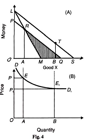
The movement from R to T is the price effect of the fall in the price of X which has resulted in its increased demand from OA to ОB. Now take away the increase in the real income of the consumer as a result of the fall in the price of X equal to LP. Thus PQ is the new price-income line which is drawn parallel to LS and passes through point R. The new triangle OPQ becomes his area of choice.
ADVERTISEMENTS:
Since the consumer was revealing his preference at point R on the original price-income line LM, therefore, all points above R on the RP segment of the line PQ are inconsistent with his choice. This is because he cannot have less quantity of good X when its price has fallen. He will, therefore, reject all combinations above R and either choose combination R or any other combination in the shaded triangle MRQ.
If the PL amount of money taken from the consumer is returned to him, he will again be at point T on the price-income line IS where he buys larger quantity OB of X than before. The movement from R to T traces out the demand curve in Panel (B) of the figure.
As we have taken money on the vertical axis in Panel (A), the price of good X can be calculated by dividing the total money income by the number of units of X bought. When the price of X is OL/OM (= OP), the quantity demanded is OA. When the price of X falls to OL/OS (=OP1), the quantity demanded increases to OB.
ADVERTISEMENTS:
In Panel (B) of the figure, we measure price on the vertical axis and units of good X on the horizontal axis and draw E and E1 price-quantity combinations. By joining these points with a smooth line, we get the demand curve DD1 .This curve shows that as price falls from OP to OP1 the consumer buys more quantity AB of X.