
In this article we will discuss about the demand function for money.
The responsiveness of the demand for money to the changes in the levels of income and the rates of interest will be very important in understanding the factors affecting the demand for money in any economy. Demand for money is concerned with the amount that would be kept in the form of cash at hand to meet various requirements. The quantity of demand for money depends mainly on transactions, precautionary and speculative motives.
Transactions and precautionary motives will be positively related to the changes in income and speculative motive will be inversely related to the changes in the rate of interest.
In empirical studies, the specification of the demand for money function will be as follows:
ADVERTISEMENTS:
Y = f [X1, X2]
Where
Y = Demand for money
X1 = Level of income
ADVERTISEMENTS:
X2 = Rate of interest [%]
A small change in X1 leads to a change in Y i.e., [ΔY/ΔX1]. This is known as the rate of change in Demand for money per a unit change in income [Marginal Effect], Similarly a small change in X2 leads to a change in Y i.e., [ ΔY/ΔX2].
This is known as rate of change in demand for money per a unit change in rate of interest [Marginal Effect],
The responsiveness of demand for money with respect to X1 [income], all else equal, will be estimated as follows:
ADVERTISEMENTS:
eY.X1 = Δ Y/ ΔX1. X1/ Y. This is known as income elasticity of demand for money.
Similarly, the responsiveness of demand for money with respect X2 [interest] all else equal, will be estimated as follows:
eY.X2 = Δ Y / Δ X2. X2/ Y. This is known as interest elasticity of demand for money.
The impact of income and interest on demand for money is empirically examined by different econometric models. The linear and log-linear forms of regression models are widely used in empirical studies.
Linear Demand Function for Money:
The specification of a linear regression model for demand for money will be as follows:
Y = b0+ b1 X1 + b2 X2+ error………………. (48)
The linear demand function for money equation will be estimated by OLS method,
Where
ADVERTISEMENTS:
b0 is the trend value of demand for money in the absence of income and interest
Partial derivate of Y with respect to X1
∂ Y / ∂X1 = b1 is the rate of change in demand for money per a unit change in X1 which is constant.
Partial derivate of Y with respect to X2
ADVERTISEMENTS:
∂ Y / ∂ X2 = b2 is the rate of change in demand for money per a unit change in X2, which is also constant
b1 will be positive [b1 > 0]
and b2 will be negative [b2< 0],
The partial elasticity of demand for money with respect to income will be evaluated at the mean values of Y and X1 as shown below:
ADVERTISEMENTS:
ey.x1 = ∂ Y / ∂ X1.X / Y = b1* mean value of X1 / mean value of Y
Since the elasticity of demand for money is estimated at the average values, it is referred to as an average elasticity of demand for money with respect to income. Sometimes, the elasticity will be evaluated from point to point, i.e., X1i and Yi.
ey.x1 = ∂ Y / ∂ X1.X1 / Yi = b1* X1 / Yi
The partial elasticity of demand for money with respect to the rate of interest will be evaluated at mean values of Y and X2 as shown below:
![]()
ADVERTISEMENTS:
Y. Hence it is referred to as an average elasticity of demand for money with respect to the rate of interest. If the elasticity is evaluated from point to point change i.e. X2i and Yi, then the equation will be:
![]()
Therefore, the elasticity of demand for money goes on changing. The numerical value of elasticity of Y with respect of X1 will be directly related to the increase in X1 and inversely related to the increase in Y, all else equal. The numerical value of elasticity of Y with respect to X2will be directly related to the increase in X2 and inversely related to the increase in Y, all else equal.
ADVERTISEMENTS:
The value of R2 will be considered for goodness of fit of the equation. If its value is high, then the equation fitted to the data points will be good. Similarly, the significant impact of X1 and X2 on Y will be considered on the basis of standard errors. If the standard errors [s.e] are less than half of b1 and b2 [ s.e. < b1/2 and s.e. < b2/2], then the impact will be statistically significant.
If the standard errors are more than half of b1 and b2 [s.e > b1/2 and s.e > b2/2] then the impact of X1 and X2 on Y will not be statistically significant. Thus, on the basis of the values of standard errors, the precision of regression coefficients can be evaluated. In empirical studies, the level of significance is evaluated either by taking standard errors or ‘t’ values.
[b1 / s.e.[b1] or b2/ s.e[b2]] at either 1% [with 99% of confidence] or 5% [with 95% of confidence] level of significance. If the linear regression model is not found to be suitable to the data points, then the other forms of equations have to be, attempted.
Log Linear Demand Function for Money:
In empirical studies, the following form of Power function [log linear regression model] will be fitted to the time series observations.
Y = b0 X1b1 X2b2
ADVERTISEMENTS:
For the purpose of estimation by OLS method, the above model is transformed into a log linear model as specified below:
log Y = log b0 + b1log X1+ b2log X2 ……………(49)
The partial derivative of log Y with respect to log X1,
∂ log Y/∂ log X1 = b1, which is partial constant elasticity of Y with respect to X1.
The partial derivative of log Y with respect to log X2,
∂ log Y/∂ logX2 = b2, which is partial constant elasticity of Y with respect to X2. The goodness fit of this equation will be considered on the basis of R2. If its value is very high, then the equation fitted to the observations gives a good fit. Since, the model is based on two independent variables, the value of adjusted R2 has to be considered.
ADVERTISEMENTS:
Short Run and Long Run Demand Functions for Money:
In empirical studies on the demand function for money, both the short-run and long-run demand functions for money are estimated through partial adjustment mechanism.
The long- run demand function for money will be specified as follows:
Yt* = b0 + b1X1t + b2X2t ……………(50)
Where
Yt* is desired level/long run level/equilibrium level/optimal level of demand for money, which is not observable.
In order to estimate the above function, the following partial adjustment mechanism is considered.
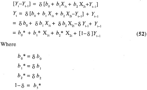
[Yt – Yt-1] = δ [Yt*-Yt-1]……………. (51)
By substituting the equation (50) in equation (51), we get the following short run
for money.
The partial derivative of Yt with respect to X1t, ∂ Y / ∂ X1t, is b1 and the partial derivative of Yt with respect to X2t, ∂ Y / ∂ X2t , is b2.
The partial elasticity of Y [demand for money] with respect to X1t ∂ Y / ∂ X1t.X1t / Y, will be as follows:
b1 * X1t / Yt, which is known as the short run income elasticity.
The partial elasticity of Y with respect to X2t, ∂ Y / ∂ X2t.X2t /Y will be as follows:
b2 * X2t / Yt, which is known as the short run interest elasticity.
The corresponding long-run income elasticity of demand for money will be estimated as follows:
SRE /δ = SRE /δ = b1X1t /Yt /δ = b2X1t / Yt* 1/δ
The long-run interest elasticity of demand for money will be estimated as follows:
SRE /δ = SRE /δ = b2X2t /Yt /δ = b2X2t / Yt* 1/δ
The long-run demand function for money can also be estimated by deflating the short-run demand function for money by δ or [1-b3*] and omitting Yt-1 term as shown below
Yt / δ = b0* / δ + b1* / δ X1t + b2* / δ X2t
If the linear form of the demand function for money is not suited to the data points, then other forms of equations have to be attempted. In empirical studies, the log linear form of the demand function for money will be attempted.
The long- run demand function in the form of log-linear function will be specified as follows:
log Yt* = log b0 + b1 logX1t + b2 logX2t ……………….(53)
Where
log Yt* is the long run/ desired/ equilibrium /optimal level of demand for money which is not observable. In order to estimate the above equation, the following partial adjustment mechanism is adopted.
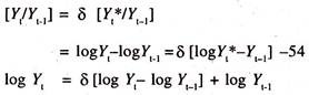
By Substituting equation (53) in equation (54) we get the following short run demand function for money
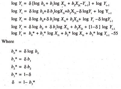
δ is the coefficient of partial adjustment between the desired change in demand for money and the actual change in demand for money. If its value is close to one, then the difference or disequilibrium between the desired change and the actual change in demand for money is quickly reduced. The partial derivative of log Yt with respect to the level of income [log X1] is b1*.
This shows the responsiveness of demand for money to the changes in the level of income, all else equal. This is also known as the short run income elasticity of demand for money. The sign of the elasticity of demand for money with respect to income will be positive.
The partial derivative of log Y1 with respect to the rate of interest [logX2] is b2*. This shows the responsiveness of demand for money to the changes in the rate of interest. This is referred to as the short run interest elasticity of demand for money.
The sign of the elasticity of demand for money with respect to the rate of interest will be negative showing an inverse association between the demand for money and the rate of interest. These elasticities are short-run elasticities i.e., the responsiveness within a period of one year. [Time period is not long enough to adjust the demand for money completely to the changes in income and rate of interest].
The long-run elasticities of demand for money with respect to income and interest [Time period is enough to adjust the demand for money completely to the changes in income and rate of interest] can be worked out by deflating the short-run elasticities with the coefficient of adjustment [δ] or regression coefficient of log Yt-1[1 –b3*]
The long-run elasticity of demand for money with respect to level of income
LRE = log Yt /log X1t/δ = b1* /δ
The long-run elasticity of demand for money with respect to the rate of interest
LRE = log Yt / log X1t / δ = b2* / δ
The long run elasticities of demand for money with respect to level of income and the rate of interest show the cumulative effect of responsiveness of demand for money to the changes in income and rate of interest over a period of time. Generally, the value of coefficient of adjustment will be less than unity. Therefore, the long-run elasticities of demand for money will be higher than that of short-run elasticities.
If the short-run elasticity of demand for money with respect to the level of income is more than unity, then it can be inferred that a one percent increase in the level of income leads to increase the demand for money by more than one percent. This shows relatively more elastic nature of demand for money.
If it is less than unity, then it can be inferred that one percent increase in the level of income leads to increase the demand for money by less than one percent. This shows relatively inelastic nature of demand for money. If it is unity, then it can be inferred that a one percent increase in the level of income leads to increase the demand for money by the same one percent, implying unitary elastic nature of demand for money.
Similarly, if the elasticity of demand for money with respect to the rate of interest is more than unity, then it can be inferred that a one percent increase in rate of interest will reduce the demand for money by more than one percent showing elastic nature of demand for money.
If it is less than unity, then it can be inferred that a one percent increase in rate of interest will reduce the demand for money by less than one percent showing an inelastic nature of demand for money. If it is unity, then it can be inferred that a one percent increase in rate of interest will reduce the demand for money by the same one percent showing unitary elastic nature of demand for money.
Since the estimation of elasticities of demand for money is based on time-series data, the problem of autocorrelation does exist. Similarly, if the movement of the variables would be in the opposite/same direction, then there will be a multi-collinearity problem.
These econometric problems affect the precision of the estimates of coefficients of the income and interest elasticities. The problem of multi- collinearity and auto-correlation can be reduced by adopting the first difference method.
ΔX1t= [X1t-X1t-1], ΔX2t= [X2t-X2t-1] and Δ Yt= [Yt-Yt-1]
The functional relationship between the first differenced variables:
ΔYt= f [ΔX1t. ΔX2t]
The linear regression model in the first difference:
[Yt-Yt-1] = b0 + b1[X1t – X1t-1] + b2 [X2t – X2t-1]
The log linear regression model in the first difference:
[log Yt– log Yt-1] = constant + b1[logX1t – logX1t-1] + b2 [log logX2t – logX2t-1
In empirical studies, apart from income and the rate of interest, other variables will also be considered to know the impact of these variables on the demand for money. It should, however, be noted that the estimation of the linear and log-linear equation by OLS method is subjected to one-way causation.
Generally, the aggregate time series variables have a unit root problem. The unit root problem (non-stationarity problem) needs to be tested. In a way, the time series properties of macro-variables have to be examined by using latest econometric techniques such as the Augmented Dicky Fuller Test (ADF) etc.,


Demand Function for Money – Estimates Economic Relationships:
The time series data given in Table 6.1 are used to explain the income and interest elasticities of demand for money.

The results of the linear demand function for money [Table 6.2] based on the data given in table 6.1 show that the regression coefficients of income and interest are significant. The income and interest average elasticities are [estimated at mean values: 0.690749*645032.4/406608.7] 1.096 and [- 5331.109* 12.6515X406608.7] -0.166 respectively.
The interest elasticity shows that if the rate of interest is increased by one percent, then demand for money comes down by 0.166 percent per annum, all else equal. The income elasticity shows that if income is increased by one percent then the demand for money goes up by 1.096 percent per annum, all else equal.

The regression results of the log linear demand function for money [Table 6.3] based on the data given in table 6.1 show that the regression coefficient of the interest rate during the period under consideration is not significant. This could be due to econometric problem of multi-collinearity between log X1 and log X2.
The regression coefficient of income is positively significant. This explains that if income is increased by one percent, then the demand for money goes up by 1.084 percent per annum, all else equal.