Income Effect and Substitution Effect | Consumption Theory

The upcoming discussion will update you about the difference between income effect and substitution effect.

It is a well-known proposition of consumption theory that a ra­tional consumer reaches equilibrium when he chooses the bundle of goods that maximises his satisfaction. He will continue to consume the goods in the proportions indicated by the point of tangency between the budget line and an indifference curve until something changes. The price-consumption line shows increasing (declining) qualities of a commodity, such as bread being bought as its price falls (rises).

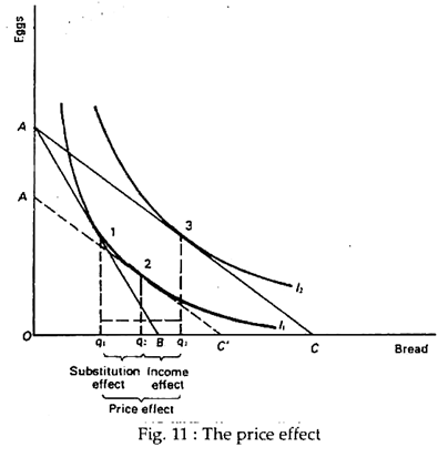
The effect of a change in the price of one of the purchasable commodities can be bro­ken down into a substi­tution effect and an income effect. In Fig. 11 we show our consumer, Ram, faced with a budget line AB. He is in equilibrium at point 1 where he consumes q, of bread. Now, let the price of bread (commodity x) fall, while money in­come and the price of eggs (commodity y) re­main the same. Ram’s new budget line is now AC and his new equilibrium is at point 3 on indifference curve h, where bread is purchased.

We may now breakdown the effect of a change in the price of bread on the quantity demanded into what J.R. Hicks called the substitution effect and income effect. The substitution effect shows the change in the consump­tion of x which occurs when its price and hence the relative prices of x and y change. When there is a change in relative price the consumer tends to substitute x (which is now relatively cheap) for y (which is now relatively expensive), although there is no change in (the absolute price of y^α).

The income effect shows the changes in quantity demanded of x resulting from the change in real income that occurs when the price of x changes (falls) while money income is held constant (by ceteris paribus assumption). A study of demand theory reveals that income changes affect demand. Now, we have to show explicitly the effect of real income changes when prices change while money income is constant, as well as when money income changes, with relatively prices held constant.

The Price Effect (or the total effect of price change):

Since price effect is the sum total of substitution effect and income effect, we can measure the size of the substitution effect by eliminating income effect. For isolating the price-substitution effect of a fall in the price of x we have to hold Ram’s real income constant and see what he would do if just relative prices changed.

The Substitution Effect:

It was Sir John Hicks who first isolated the pure substitution effect of the price change in the following manner. Following Hicks, we hold the con­sumer’s real income constant, and see what he would do if just relative prices changed. If the consumer’s real income remains unchanged he will stay on the old indifference curve h, and continue to enjoy the same level of satisfaction or utility as before the change in relative price.

However, he will not maximise satisfaction at point 1, because there has occurred a change in relative price. The relative price is no longer given by the slope of the line AB, but by the slope of the line AC. So, to find out the best combination of eggs and bread we try to find where on his indifference curve Ii he will settle. The answer is that, he will select the point on the curve where the new relative price of bread in terms of eggs is equal to MRS.

This occurs where the indifference curve is tangent to the line representing the ratio: the price of bread – the price of eggs. To find this line we construct the line A’ C’, parallel to AC, and also tangent to h. Since A’ C’ and AC are parallel, they have the same slope; and since the point of tangency of A’ C with I₁ is the consumer’s equilibrium point, he will surely maximise satis­faction (or reach the point of maximum welfare) at point 2.

This shows that his equilibrium purchase of bread is q₂, if the price of bread falls and consumer’s real gain is eliminated. His real income gain is eliminated by a parallel shifting of the budget line AC to the left to A’ C in such a fashion that it is tangent to the old indifference curve h.

This implies that the consumer is just enable to enjoy the same (old) level of satisfaction at the new set is q₁q₂. This is the substitution effect of a change in the price of bread. In short, substitution effect measures the change in the consumption of bread that occurs when the consumer moves along the same indifference curve due to a fall in the market price of bread.

The Income Effect:

Since we have a clear idea of the total effect of the price change, we can easily determine the size of the income effect. Recall that the price effect is the sum of the income and substitution effects. Since we have already measured the substitution effect we can now deduce the size of the income effect imme­diately as q₃-q₂ bread.

It is just the difference between the total income in quantity q₃-q₂ minus the substitution effect of q₂-q₁ bread. However, it is both important and interesting, at least from the conceptual point of view, to understand how the income effect is (formally) derived. Simply put, the (pure) income effect of a price change is the extent to which a change in real income affects the quantity demanded of bread, with relative price held constant.

While isolating the substitution effect we held real income constant by confining the consumer to his old (original) indifference curve, I₁. Now, in order to identify and measure the income effect we remove this restriction and allow the consumer to reach a higher indifference curve (l₂). In other words, we shift the budget line A’ C’ back to the position AC.

This enables the consumer to reach the higher indifference curve I₂ and enjoy a higher level of satisfaction or utility at point 3. So, point 3 is his new equilibrium point after the restoration of the income effect. In fact, we eliminated the income effect by shifting the budget line AC to the left to A’ C. Now, that we have been able to measure the size of the substitution effect, we follow an exactly opposite procedure. We shift the budget line back to the position AC.

Since we are now only interested in the income effect of the price change, we have to observe the behaviour of the consumer when we allow his income to rise, with no change occurring in relative price.

In order to isolate income effect we have just to observe the difference in the consumer’s consumption of bread when the price of bread is held constant, but his real income is allowed to rise as much as it would from the fall of price (of bread). To do this we have to hold the market prices of the two goods constant and raise his real income.

Differently put, all we have to do is to compare his consumption of bread at point 3 with that at point 2, because the relative price of bread is the same at both points. Only his real income has increased so as to enable him to move from I₁ to I₂.

From Fig. 11 we observe that our consumer increases his consumption of bread from q₂ to q₃ when the price of bread is held constant but his real income rises. Thus q₃-q₂ measures the income effect of the price change. In short, the income effect measures the change in the consumption of bread that occurs when the consumer moves to a higher indifference curve (representing the change in real income).

Price Effects with Inferior and Giffen Goods:

In dividing the price effect into two parts we assumed that bread was a normal and not an inferior good.

Normal goods, it may be recalled, are those for which the quantity demanded by a consumer rises when income rises and falls when income fall. In case of normal goods both the income effect and substitution effect move in the same direction. From Fig. 11 we see that bread being a normal good, the fall in its price led the consumer to buy more of it as a result of consumer’s real income gain. The substitution effect also led to an increase in consumption of bread.

In the case of inferior goods the two effects of price change actually work in opposite directions. The substitution effect is always negative. It is because holding the real income constant; the consumer will always tend to substitute a good whose price has fallen for one whose price remains the same. But, income effect is positive in case of normal goods and negative in case of inferior goods.

In case of normal goods the income effect reinforces the substitution effect. But, in case of an inferior good, income effect operates in the opposite direction to the substitution effect. If the price of an inferior good falls the substitution effect will still cause a larger commodity. This is because the fall in price raises the real income of the consumer. This, for an inferior good, means that les§ will be purchased, when price falls.

Economic theory cannot tell us whether the income effect or substitution effect will predominate. It is a matter of empirical research. However, we can consider the following two possibilities.

Case 1: Inferior Goods: The Substitution Effect Exceeding the Income Effect:

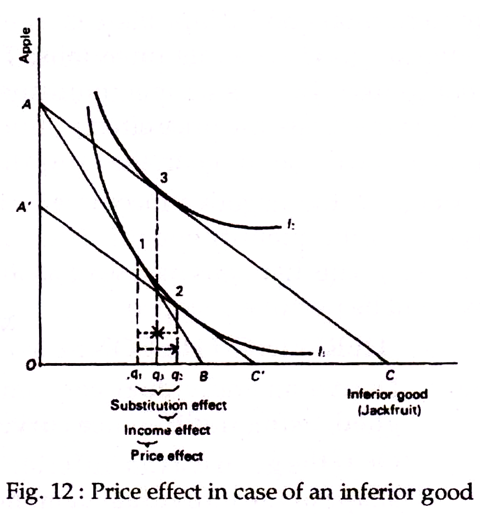
In Fig. 12 we show that the substitution effect is stronger than the income effect. Here apple is a normal good and jackfruit is an inferior good. The consumer’s equilibrium is at point 1. He buys q₁ units of jackfruit. The price of jackfruit now falls. This is indicated by the shift of the budget line from AB to AC. Now, the substitution effect shifts the consumer from point 1 to 2.

As a result of this there is an increase in the quantity bought of q₂-q₁. However, as a result of income effect, equilibrium moves from point 2 to point 3. Because jackfruit is as­sumed to be an inferior good, there is a fall in the quantity demanded of (q₂-q₁), due to in­come effect alone. The net effect (or full price effect) is an in­crease in quantity of jackfruit bought of q₃-q₁. This is made up of an increase in q₂-q₁ (sub­stitution effect) and a decrease of q₂-q₃ (income effect). The substitution effect is greater (stronger) than the income ef­fect.

  Case 2: Giffen Goods: The Income Effect Exceeding the Substitution Effect:

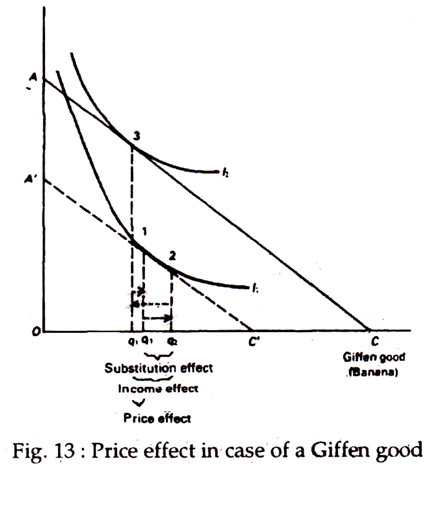
Fig. 13 illustrates the case of a special variety of inferior good, known as Giffen good, in which case the income effect is stronger than the substitution effect. In Fig. 13, the original equilibrium is at point 1 with quantity q₁ consumed. Now, the fall in price of the Giffen good shifts the budget line from A B to AC as usual.

The substitution effect is also the same as before q₂-q₁. The consumer buys more of the Giffen good due to substitution effect. But, income effect in this case is q₂-q₃, which is so large that it outweighs the income effect. So, the net effect of a fall in the price of a Giffen good is a fall in the quantity demanded.

Fig. 12 and 13 show price effect for inferior goods. The income effect is negative in both the diagrams. This follows from the very definition of an inferior good: an inferior good is one the quantity demanded of which falls when income rises.

In each case, the substitution effect serves to increase the quantity demanded as price falls and is partly offset by the negative in­come effect. The net effect of price change depends on the relative strengths of the two ef­fects. In Fig. 13 the negative in­come effect is less strong than the substitution effect. So the quantity demanded of an infe­rior good increases when its price falls, though not as much as for a normal good.

 

Thus, there is a net income in the quantity bought of an inferior good when its price falls. This produces a negatively sloped demand curve. But it is stepper (more inelastic) than that in case of a normal good, in which case the price effect is much strong (since its two components reinforce each other or go in the same direction).

In Fig. 13, the negative income effect is stronger than the substitution effect. Thus, the quantity bought of the commodity falls (rises) when its price falls (rises). This happens in case of a Giffen good. In this case, the demand curve will be positively sloped.