National Income and Consumption and Saving Functions

The following article will guide you to learn how national income determines consumption and saving functions.

Although national income accounting provides estimates of the nation’s output, it does not explain why the nation’s output is at a certain level or why it increases more rapidly in some years than in others.

In a simple Keynesian model aggregate demand — the sum of society’s expenditures on consumption and investment — determines the equilib­rium level of income. If aggregate demand changes, the equilibrium level of income also changes.

The Consumption Function:

Many different factors, including tastes and preferences, income and inter­est rates, determine consumption. For example, if the income of one house­hold is greater than the income of another, the former is likely to consume more.

Even if their incomes are the same, however, they will spend different amounts on consumption if their attitudes toward thrift differ. Similarly, households vary their consumption in response to changes in interest rates.

Although many factors affect consumption, aggregate income in the most important by far. Consequently, we shall concentrate on the relationship between consumption and income, called the consumption function.

In Keynesian consumption function, consumption is assumed to vary directly with income. Specifically, consumption is assumed to increase with income, with the increase in consumption being less than the increase in income.

The consumption function is expressed as:

C = a + bY (a > 0, 0 < b < 1).

where C and Y represent real consumption and real income, respectively. The equation indicates that consumption is a linear function of income. In the equation, ‘a’ and ‘b’ are constants, called parameters. Consumption, C, and income, Y, are variables.

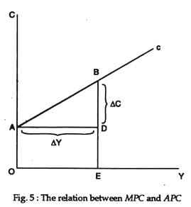
The parameter b, called the marginal propensity to consume or MFC, is the slope of the consumption function. If ΔY denotes a change in income and ΔC denotes the change in consumption associated with the change in income, b, the MPC, equals ΔC/ΔY.

For example, if income increases by Rs 200 crores and, as a result, consumption increases by Rs 150 crores, the MPC is Rs. 150 crores divided by Rs. 200 crores or 0.75. In postulating his consumption function, J.M. Keynes assumed that consumption increases as income increases, but by a smaller amount. Thus implies that b, the MPC, must lie between 0 and 1.

The parameter a is the portion of consumption which does not vary with income, i.e., a represents the consumption which would occur if income were 0. Short-run studies of the consumption function show that a is positive.

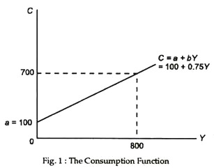
The consumption func­tion may be shown graphi­cally by specifying various levels of income, determin­ing the corresponding levels consumption, and then plotting the combina­tions of income and con­sumption. To illustrate, suppose the consumption function is C = 100 + 0.75Y.

If Y equals Rs 100 crores, C equals Rs 700 crores, ob­tained by solving the equa­tion C = 100 + 0.75 (800). This combination of Y and C is plotted as a point on the consumption function C = 100 + 0.75Y in Fig. 1. Other points on the consumption function can be obtained in the same way.

An alternative way to plot the consumption function is to recognise that ‘a’ is the intercept and b the slope. Once the intercept and slope are specified, a straight line is completely determined. For example, if ‘a’ equals 100 and b equals 0.75, the function will start at a = 100 and have a slope, b, equal to 0.75. If a changes, the consumption function will shift so that the new function is parallel to the old. If b changes, the function will change its slope. It may become flatter or steeper.

The Saving Function:

Since the decision on how much income to consume implies a decision on how much to save, a saving function may be derived with the aid of the consumption function.

With no government and foreign trade sectors, income equals, by definition, consumption plus, saving, S:

Y = C + S

But C is equal to a + bY. Consequently, after substituting, the saving function is found to be

S = -a + (1 – b ) Y (0 < 1 – b < 1)

where S and Y represent real saving and real income, respectively.

The parameter 1 – b, referred to as the marginal propensity to save or MPS, is the slope of the saving function. If ΔY denotes a change in income and ΔS denotes the change in saving associated with the change in income, 1 – b, the MPS, equals ΔS/ΔY.

For example, if income increases by Rs 200 crores and, as a conse­quence, saving in­creases by Rs. 50 crores, the MPS is Rs 50 crores divided by Rs 200 crores or 0.25. Since b, the MPC, is as­sumed to be between 0 and 1, 1 – b, the MPS, is also between 0 and 1, which implies that saving increases as in­come increases, but by a smaller amount.

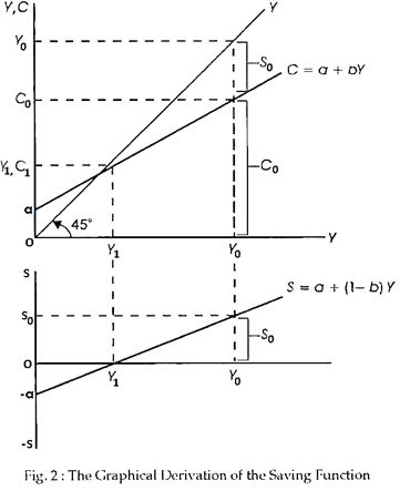
The saving func­tion may be plotted in the same manner as the consumption function. To show the relationship between the consumption and saving functions, however, we may consider an alterna­tive approach. Sup­pose, in Fig. 2, income is plotted on both axes and that a 45° line is drawn through the origin.

At all points on the 45° line, income on the vertical axis is equal to income on the horizontal axis. Given the 45° line and the consumption function, we can now derive the saving function graphically. Since income equals consumption plus saving, saving is the difference between income and consumption. Therefore, to find saving at each level of income, consumption is subtracted from income.

Graphically, saving is the vertical distance between the income line, the 45° line, and the consump­tion function, saving being positive (negative) when income is greater (less) than consumption. Consider income Y₀ in Fig. 2. At income Y₀, consumption equals C₀; consequently, saving equal S₀, obtained by subtracting C₀ from Y₀. Therefore, one point on the saving function is the point Y = Y₀, S = S₀.

Let us select another level of income, say, Y₁ where the consumption function intersects the 45° line. At that level of income, consumption equals C₁, which also equals Y₁. Therefore, at Y = Y₁, S₁ equals 0, since S₁ equals Y₁ – C₁ and C₁ equals Y₁. Consequently, another point on the saving function is the point Y = Y₁, S = 0.

Finally, suppose income is 0. At that level of income, consumption equals a. Hence, saving equals -a, obtained by subtracting C = a from Y = 0. Thus, a third point on the saving function is the point Y = 0, S = -a. Other such points may be obtained by considering other levels of income.

In Fig. 5, saving is positive at income levels greater than Y₁, since income exceeds consumption at those levels of income. Saving is negative at income levels less than Y₁ since consumption exceeds income. Negative saving, dissaving, occurs if individual households consume more than their in­come. They may do so by spending part of their savings or by borrowing. For society as a whole, dissaving is unlikely.