According to Keynes, there can be different sources of national income, such as government, foreign trade, individuals, businesses and trusts.
For determining national income, Keynes had divided the different sources of income into four sectors namely’ household sector, business sector, government sector, and foreign sector.
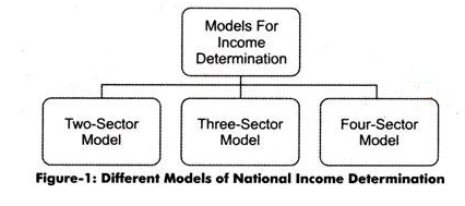
He prepared three models for the determination of national income, which are shown in Figure-1:
The two-sector model of economy involves households and businesses only, while three-sector model represents households businesses, and government. On the other hand, the four-sector model contains households, businesses, government, and foreign sector.Let us discuss these three types of models of income determination given by Keynes.
ADVERTISEMENTS:
Determination of National Income in Two-Sector Economy:
The determination of level of national income in the two-sector economy is based on an assumption that two-sector economy is an economy where there is no intervention of the government and foreign trade.
Apart from this, an economy can be a two-sector economy if it satisfies the following assumptions:
ADVERTISEMENTS:
a. Comprises only two sectors, namely, households and businesses. The households are the owners of factors of production and provide factor services to businesses to earn their livelihood in the form of wages, rents, interest, and profits. In addition the households are the consumers of final goods and services produced by businesses. On the other hand, businesses purchase factor services from households to produce goods and services and sell it to households.
b. Does not have government interference. If government is there, it does not have any role to play in the economic activity of a country. For example, in the two-sector economy, the government is not involved in activities, such as taxation, expenditure, and consumption.
c. Comprises a closed economy in which the foreign trade does not exist. In other words, import and export services are absent in such an economy.
d. Contains no profit that is undistributed or savings by the organization. In other words, the profit earned by an organization is completely distributed in the form of dividends among shareholders.
ADVERTISEMENTS:
e. Keeps the prices of goods and services, supply of factors of production, and production technique constant throughout the life cycle of organization.
Keynes believed that there are two major factors that determine the national income of a country. These two factors are Aggregate Supply (AS) and Aggregate Demand (AD) of goods and services.
In addition, he believed that the equilibrium level of national income can be estimated when AD=AS. Before representing the relationship between AS and AD on a graph, let us understand these two concepts in detail.
Aggregate Supply:
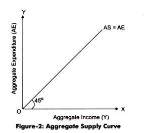
AS can be defined as total value of goods and services produced and supplied at a particular point of time. It comprises consumer goods as well as producer goods. When goods and services produced at a particular point of time is multiplied by the respective prices of goods and services, it provides the total value of the national output. The national output is the aggregate supply in the form of money value. The Keynesian AS curve is drawn based on an assumption that total income is equal to total expenditure. In other words, the total income earned is fully spent on different types of goods and services.
The correlation between income and expenditure is represented by an angle of 45°, as shown in Figure-2:
According to Keynes theory of national income determination, the aggregate income is always equal to consumption and savings.
The formula used for aggregate income determination:
ADVERTISEMENTS:
Aggregate Income = Consumption(C) + Saving (S)
Therefore, the AS schedule is usually called C + S schedule. The AS curve is also named as Aggregate Expenditure (AE) curve.
Aggregate Demand:
AD refers to the effective demand that is equal to the actual expenditure. Aggregate effective demand refers to the aggregate expenditure of an economy in a specific time frame. AD involves two concepts, namely, AD for consumer goods or consumption (C) and aggregate demand for capital goods or investment (I).
ADVERTISEMENTS:
Therefore, the AD can be represented by the following formula:
AD = C + I
Therefore, AD schedule is also termed as C+I schedule. According to Keynes theory of national income determination in short-run investment (I) remains constant throughout the AD schedule, while consumption (C) keeps on changing. Therefore, consumption (C) acts as the major determinant or function of income (Y).
The consumption function can be expressed as follows:
ADVERTISEMENTS:
C = a + bY
Where, a = constant (representing consumption when income is zero)
b = proportion of income consumed = ∆C/∆Y
By substituting the value of consumption in the equation of AD, we get:
AD = a + bY + I
Let us prepare an AD schedule by assuming that the investment is Rs. 50 billion and consumption function of a product is:
ADVERTISEMENTS:
C = 50 + 0.5 Y
Therefore, aggregate demand would be:
AD = a +b Y + I
AD = 50 + 0.5 Y + 50
AD= 100 + 0.5 Y
The aggregate demand schedule at different income levels is represented in Table-1:
In Table-1, the column of income represents the aggregate supply and the column of aggregate demand represents expenditure. In Table-1, it can be noticed that at Rs. 200 billion of income level, aggregate supply and aggregate demand are equal. Therefore, Rs. 200 billion is the equilibrium point for the two-sector economy.
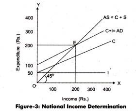
Figure-3 represents the graphical representation of national income determination in the two-sector economy:
In Figure-3, while drawing AS schedule it is assumed that the total income and total expenditure are equal. Therefore, the numerical value of AS schedule is one. AD schedule is prepared by adding the schedule of C and I. The aggregate demand and aggregate supply intersect each other at point E, which is termed as equilibrium point.
The income level at point E is Rs. 200 billion, which represents the national income of the economy. The schedule curve after point E represents that the AS is greater than AD (AS > AD). In such a situation, the products and services are costing more than Rs. 200 billion; therefore, households are not willing to buy them.
Therefore, the supply of products and services exceeds their demand. As a result, businesses would have a pile of unsold stocks. For example, in Table-1, when the income or aggregate supply is at Rs. 300 then the aggregate demand or expenditure is Rs. 250, which is less than the aggregate supply.
ADVERTISEMENTS:
Similarly, beneath point E, the AD and AS schedules represent that the aggregate demand is more than aggregate supply. In such a case, the production by businesses is less than the demand of households. Therefore, businesses start producing more and more products and services. For example, in Table-1, when the income or aggregate supply is Rs. 100 then the aggregate demand is Rs. 150, which is more than the aggregate supply.
The equilibrium condition of national income determination can be expressed as follows:
Aggregate demand = Aggregate supply
C + I = C-HS
Therefore, I = S
Thus, the national income can be determined by using either aggregate demand and aggregate supply schedules or investment and savings schedules. These two methods of income determination are classified as income-expenditure approach and saving- investment approach.
ADVERTISEMENTS:
Income-Expenditure Approach:
Income-expenditure approach refers to the method in which the aggregate demand and aggregate supply schedules are used for the determination of national income.
In this method, the equilibrium point is achieved when the following condition is satisfied:
C+I=C+S
As, C + S = Y, therefore, the equilibrium condition of national income determination would become:
Y = C + I
At equilibrium point, the consumption is equal to:
C = a + bY
Substituting the value of C in the national income equilibrium condition, we get:
Y = a + bY + I
Or, Y (1- b) = a + I
Thus, Y = 1/1-b (a + I)
For the determination of national income with the help of income-expenditure approach, let us assume that the consumption function is C = 200 + 0.50Y and I = 150.
In such a case, the national income can be calculated as follows:
Y = C + I
Y = 200 + 0.50Y+ 150 1
Y = 1/1-0.50(200 + 150)
Y = 1/1.50(350)
Y = 700
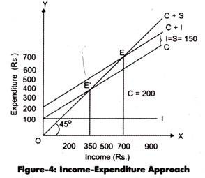
Therefore, the national income equilibrium in this case is at Rs. 700. The graphical representation of national income determination with the help of income-expenditure approach is shown in Figure-4:
In Figure-4, the schedule of C + S shows the aggregate supply of income while the C + I schedule denotes the aggregate demand. Aggregate demand schedule is drawn by adding C and I schedules. Aggregate demand and aggregate supply schedule intersect each other at point E and the Income level at this point is Rs. 700.
This implies that the national income in the two-sector economy is Rs. 700. In short-run, the equilibrium point remains constant that is the level of national income remains constant. If there is any type of increase or decrease in the aggregate supply/demand, then they themselves fluctuate in a manner, so that they reach back at the equilibrium point.
Saving-Investment Approach:
Saving-investment approach refers to the method in which the saving (S) and investment (I) are used for the determination of national income. The condition for achieving equilibrium with the help of saving-investment approach is that the saving and investment are equal (I = S).
Let us take the previous assumption that consumption function is equal to C = 200 + 0.50 Y and I = 150 for the determination of national income by using the saving-investment approach.
In such a case, the saving function can be determined as follows:
Y = C + S
Or,
S = Y-C
S = Y – (a + bY)
S = Y – a – bY
S = -a + (l-b) Y
Therefore, in the present case, the saving function would be:
S = -200 + (1 -0.50) Y
S = – 200 + 0.50 Y
At equilibrium point I = S, therefore, the national income equilibrium would be:
150 = -200 + 0.50 Y
Y= 700
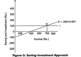
The national income level at equilibrium point is same in both the cases, income-expenditure approach and saving-investment approach. Figure-5 provides a graphical representation of national income determination by using the saving-investment approach:
In Figure-5, equilibrium point is at E where the investment and saving curve intersects each other. The national income at equilibrium level is Rs. 700.
Shifts in Aggregate Demand Schedule:
In the above, you have learned to determine the equilibrium level of national income under a given AD schedule that is C+I. A shift in aggregate demand schedule can produce changes in the equilibrium level of national income in the two-sector economy. Therefore, it is necessary to study and understand the shifts that arise in AD schedule and determine measures to get the equilibrium position back. In a two-sector economy, a shift in AD schedule occurs due to a shift in consumption or investment schedule or in both, simultaneously.
However, shifts in consumption schedule are very rare as it is an income function, whereas investment schedule can fluctuate because of autonomous factors, such as risks and individual perceptions. Therefore, the shift in AD schedule is because of the shifts in investment schedule.
For understanding the impact of shift in AD schedule on equilibrium point, let us assume that the AD schedule is showing an upward shift due to a permanent upward shift in the investment schedule. The investment schedule is shifting due to the autonomous investment in some venture. As a result, the equilibrium point also shifts in the upward direction and the national income also increases.
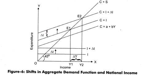
Figure-6 demonstrates the shift in national income due to shift in equilibrium point and AD schedule:
In Figure-6, C + I schedule represents the initial AD schedule. The initial equilibrium is at point E, where C+S schedule or AS schedule intersects AD schedule and the level of national income is Y1. Suppose investment increases, which leads to a movement in the investment schedule from I to I + ΔI, showing an upward shift. Consequently, the AD schedule also moves from C + I to C + I + ΔI. With the shift in AD schedule, the equilibrium point reaches to E2 and level of national income reaches to Y2.
The increase in national income can be calculated as follows:
ΔY = Y2 –Y1
The national income increases due to increase in the investment. Let us determine the relationship between change in national income (ΔY) and change in investment (ΔI) by understanding the concept of multiplier given below.
Concept of Multiplier:
The concept of multiplier can be understood by determining the relationship between change in national income (ΔY) and change in investment (ΔI).
According to Figure-6, at equilibrium point E1, the national income is as follows:
Y1 = C + I
The consumption is equal to:
C = a + bY
By substituting the value of C in the equation of national income at point E1, we get:
Y1 = a + bY1 + I
Y1 = 1/1-b (a + I)
Similarly, at equilibrium point E2, the national income would be:
Y2 = C + I + ΔI
Y2 = a + bY2 + I + ΔI
Y2 = 1/1-b (a + I + ΔI)
By subtracting Y1 from Y2, we get:
ΔY = 1/1-b (a + I + ΔI ) – Y2 = 1/1-b (a + I)
ΔY = 1/1-b ΔI
The preceding equation of ΔY determines the relationship between ΔY and ΔI. It implies that ΔY is 1/1-b times of ΔI and 1/I-b is termed as multiplier (m).
The formula used for calculating multiplier is as follows:
ΔY/ΔI = 1/1-b
So, m = 1/1-b
In mathematical terms, the multiplier is defined as the ratio of change in national income that occurs due to change in investment. It is also termed as investment multiplier because change produced in national income is due to change in investment.
As discussed earlier that b can be calculated with the help of the following formula:
b = ΔC/ΔY
This is the equation of Marginal Propensity to Consume (MPC). Therefore:
MPC = b = ΔC/ΔY
Thus, it can be said that MPC is the determinant of multiplier value. The value of multiplier would be higher if the value of MPC is greater.
The relationship between m and MPC can be represented as follows:
m = 1/1-b
m = 1/1-MPC
Table-2 represents the value of multiplier for different values of MPC:
Multiplier can also be calculated with the help of Marginal Propensity to Save (MPS).
So, the formula for calculating multiplier with the help of MPS is as follows:
m = 1/MPS = 1/1-MPS
Therefore, multiplier can also be termed as the reciprocal of MPS.
The multiplier can be of two types on the basis of its application.
The two types of multiplier are explained in the following points:
(a) Static Multiplier:
Refers to a multiplier in which it is assumed that the change in investment and income are simultaneous. There is no time lag between change in investment with respect to change in income. For example, in Figure-6, the shift in the equilibrium position from E1 to E2 is the result of change in investment (ΔI) without any time lag.
In case of static multiplier, when the equilibrium position shifts from one point to another, the aggregate MPC does not show any change. In addition, it is also assumed that the consumer tastes and preferences and income distribution remains constant. It is also called comparative static multiplier, simultaneous multiplier, logical multiplier, timeless multiplier, and lagless multiplier.
(b) Dynamic Multiplier:
Refers to the multiplier that analyzes the movement of equilibrium position from one point to another. In a logical sense, there is a time gap between an increase in income with the corresponding increase in autonomous investment. The income cannot rise immediately when an autonomous investment is made because there is always a time lag in increase in income and consumption expenditure.
Let us understand the process of dynamic multiplier with the help of an example. Suppose the autonomous investment increases by Rs. 100 and MPC is equal to 0.8, with no expenditure, except consumption expenditure.
The increase in investment would result in the equal increase of income, which is described as follows:
ΔI = 100 = Δy1
When the income of individuals increases to Rs. 100, the consumption expenditure is Rs. 80(= 100*0.8) Now, the expenditure of Rs. 80 would become the income for suppliers; therefore, an additional income for suppliers would be Δy2 = Rs. 8o. Consequently, suppliers would spend Rs. 64 (=80*0.8).
This produces an additional income for suppliers of consumer goods and services that is’ equal to Δy3 = Rs. 64. The additional income continues to produce till the value of change in income. Δy reaches to zero. In the process, the value of Δy decreases continuously from Δy1 > Δy2 > Δy3 to Δyn-1.
The calculation of ΔY is shown as follows:
ΔY= Δy1 + Δy2 + Δy3 + Δy4 … Δyn-1
ΔY = 100 + 100 * (0.8) + 100 * (0.8)2 + 100 * (0.8)3……. + 100 * (0.8)n-1
ΔY = 100 + 80 + 64 + 51.20………→ 0
ΔY= 500
The value of multiplier can be obtained by using the following formula:
m = ΔY/ΔI
m = 500/100
m = 5
The series of national income can be generalized as follows:
ΔY = Δy + Δy (b) + Δy (b) 2 + Δy (b) 3………… Δy (b) n-1
ΔY= Δy (1 + b + b2 + b3 …………….. bn-1)
ΔY = Δy 1/1-b
As Δy = ΔI; therefore, the formula of national income can also be written as follows:
ΔY = ΔI1/1-b
Thus, the formula of dynamic multiplier is as follows:
m = ΔY/ΔI = 1/1-b
Limitations of Multiplier:
Apart from its important uses in macroeconomics, the multiplier also has certain limitations.
Some of the limitations of multiplier that need to be considered while using the concept are as follows:
(a) Based on MPC:
Refers to the main limitation of multiplier. The value of multiplier depends upon the rate of MPC. Therefore in case the rate of MPC is lower, the value of multiplier would also be lower. Generally as compared to developed countries rate of MPC is higher in developing countries or less developed countries. Therefore, the value of multiplier is also higher in developing countries. However, it is not true in practical situations.
(b) Assumption of income and investment:
Refers to the fact the theory of multiplier is based on an assumption that additional income earned by individuals as a result of some autonomous investment is spent on the consumption of goods and services only which is not the real concept. Individuals can spend their additional income on various resources, such as clearing dues buying second-hand goods, and purchasing imported goods and shares and debentures.
All these resources are termed as leakages in the flow of consumption, which adversely affect the rate of multiplier. For example suppose Mr. A earns Rs. 1, 00,000 from a contract. He pays money to the creditor, Mr. B of his contract. Mr. B buys a second hand car with that amount from Mr. C. Further, Mr. C deposits the money in a foreign bank.
In this way, the money circulates but the demand for new consumer goods and services is not generated. In such a case, the rate of multiplier would be one. The other forms of leakages are idle cash and foreign deposits.
(c) Assumption of adequate supply:
Refers to another major limitation of multiplier. The theory of multiplier is based on an assumption that goods and services are abundant and there would be no scarcity of them in economy. However if there is a situation of scarcity in the economy, then the consumption expenditure would automatically be reduced, irrespective of the rate of MPC.
As a result, the multiplier also reduces. On the contrary, if consumption expenditure keeps on increasing, it would result in inflation, while there would be no increase in the real income.
(d) Not Applicable under the condition of full employment:
Implies that the theory of multiplier does not work in the situation of full employment. This is because in case of full employment there is no scope of producing additional goods and services and generating additional real income.
