Tax Multiplier of National Income (With Example)

Let us learn about Tax Multiplier of National Income.

We have seen earlier that a tax increase results in a decline in income. In other words, it is contractionary in effect. An increase in tax (∆T) leads to a decrease in income (∆Y). The ratio of ∆Y/∆T, called the tax multiplier, is designated by K_T.

Thus,

K_T = ∆Y/∆T and ∆ Y = K_T. ∆ T

Again, how much national income would decline following an increase in tax receipt depends on the value of MPC:

The formula for K_T is:

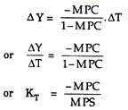
Thus, tax multiplier is negative and, in absolute terms, one less than government spending multiplier. If MPC = ¾ then the value of K_T = (-3/4)/ (1 – 3/4) = – 3. This means that an increase in taxes of Rs. 20 crore results in a decline of income of Rs. 60 crore.

That is to say

60 = (-3/4)/(1 – 3/4). 20

In contrast, with an MPC = 3/4, the value of K_G = 4. Assume an increase in government expenditure of Rs. 20 crore.

Applying the formula for K_G, we obtain:

∆ Y = 1/1 – MPC. ∆G

80 = 1/ 1 – 3/4. 20

∆Y/∆G = 80/20 = 4

Thus, K_T is negative and its value is one short of K_I or K_G.

Graphically, tax multiplier has been shown in Fig. 10.18. Pre-tax consumption line and aggregate demand schedule are represented by C_I and C_I + I̅ + G̅, respectively.

The corresponding level of income is OY₁. An increase in taxes shifts consumption line to C₂. Consequently, aggregate demand schedule also shifts downwards to C₂ + I̅ + G̅. Consequently, income declines to OY₂. Thus the effect of an increase in taxes on income is contractionary.

One must know the distinction between K_I or K_G and K_T. This is demonstrated in Table 10.4.

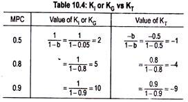
Thus, K_T is negative and one less than K_I or K_G.

The G-multiplier and the T-multiplier are also called fiscal multipliers as these multipliers are associated with the fiscal activities of the government (i.e., changes in expenditure and taxation plans).