Perfectly Competitive Market Equilibrium (With Diagram)

The below mentioned article provides an overview on the Perfectly Competitive Market Equilibrium.

A perfectly competitive market is one in which the number of buyers and sellers is very large, all engaged in buying and selling a homogeneous product without any artificial restrictions and possessing perfect knowledge of market at a time.

There are two parties which bargain in such a market, the buyers and the sellers. It is only when they agree; a commodity can be bought and sold at a certain price. Thus product pricing is influenced both by buyers and sellers, which is by demand and supply.

The law of demand is applicable to buyers. According to this, when price rises, demand falls and vice versa the law of supply applies on the supply side. This law states that supply increases with the rise in price, and decreases with the fall in price. Thus demand and supply are the two counteracting forces which move in the opposite directions.

Price is determined at a point where these two forces are equal, and that is known as the equilibrium price. Quantity demanded and supplied at this price is called the equilibrium quantity. When price is less or more than the equilibrium price, there is disturbance in the equilibrium output. But ultimately equilibrium price will prevail. This pricing process is explained in terms of Table 1 and Figure 1.

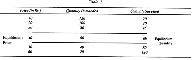
The demand and supply schedule of apples is shown in the above Table. When the price of apples is Rs.10 per kg 120 kg. of apples are demanded and 20 kg. are supplied. With the rise in price, demand is falling and supply is increasing.

When the price of apples is Rs.40 per kg., both demand and supply are 60 kg. This is the equilibrium quantity which has been determined by the equilibrium price of Rs.40. Once the equilibrium price is established, there is no tendency for it to change.

If at any time, price becomes lower or higher than Rs.40, the forces of demand and supply will bring it back to Rs.40. For instance, if the price falls from Rs.40 to Rs.30, the demand rises to 80 kg. and the supply decreases to 45 kg. Less supply of apples in relation to higher demand for them will raise the price to Rs.40. As a result, the demand will fall to 60 kg, and the supply will also increase to 60 kg.

Thus the equilibrium price is re-established. On the contrary, with the price rises to Rs.50, demand falls to 40 kg. and supply increases to 80 kg. When every seller tries to sell his product (apples) first, he has to lower his price a little and others also follow him till the price comes down to Rs.40 and the equilibrium between demand and supply is re-established.

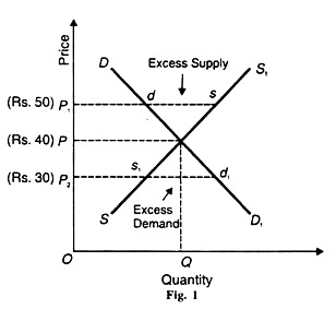
In Figure 1, equilibrium price and output are shown. (Rs.50) p DD₁ is the demand curve and SS₁ is the supply curve.

Both intersect at E which is the equilibrium point. OP is the equilibrium price at which OQ equilibrium quantity is bought and sold. If the price falls from OP to OP₂, demand P₂d > P₂s₁ supply and s₁d₁ represents the excess demand. Since demand is greater than supply, competition among buyers will raise the price from OP₂ to the equilibrium price OP.

If the price rises from OP to OP₁ supply P₁S > P₁d demand which leads to an excess supply of ds quantity in the market. Since demand is less than supply, every seller will try to sell his quantity of the product first by lowering the price a little. Ultimately, competition among sellers will bring down the price to the equilibrium level.

Thus price is determined by demand and supply and once the equilibrium price is established, any deviation from this level will be restored by the automatic forces of demand and supply.

Changes in Demand and Supply:

We studied static equilibrium in the above analysis by assuming unchanged demand and supply. But in reality, changes in demand or supply or in both bring about changes in equilibrium price and quantity, and at every change a new equilibrium position is established. The effects of changes in demand and supply on the price and quantity of a product are explained with the help of figures.

Effects of Changes in Demand:

Changes in demand are due to changes in tastes, income and preferences of consumers, etc.

The effects of changes in demand are shown in Figure 2 where D and S are the demand and supply curves respectively which intersect at E and establish OQ equilibrium quantity at OP equilibrium price. Given the supply if the demand rises, the demand curve shifts upward as D₁ which intersects the supply curve S at E₁ .The equilibrium price rises form OP to OP, and the equilibrium quantity from OQ to OQ₁.

On the contrary, with the fall in demand the demand curve D shifts downward as D and intersects the supply curve S at E₂ As a result, the price falls from OP to OP₂ and quantity from OQ to OQ₂. Thus, given the supply, rise in the demand of the product raises both the price and the quantity, and vice versa.

If the supply curve is elastic, a change in demand brings about a smaller change in price and a larger change in quantity. In Figure 3 (A), S is an elastic curve. With the upward or downward shift in D to D, or D₂, the change in price from OP to OP₁ or OP₂ is less than the change in quantity from OQ to OQ, or OQ₂.

On the contrary, if the supply curve is less elastic a change in demand leads to a larger change in price and a smaller change in quantity.

Such a situation is shown in Figure 3 (B) where S is the less elastic supply curve with the change in demand from D to D₁ or D₂, the change in price from OP to OP, or OP₂ is greater than the change in quantity from OQ to OQ₁ or OQ₂.

Effects of Changes in Supply:

Changes in supply are due to changes in technical knowledge and factor prices. Figure 4 shows the effect of changes in supply. Given the demand when the supply increases, the supply curve shifts downward to the right. As a result the price of the product falls and its quantity increases. Taking S and D as the supply and demand curves respectively, they intersect at E and establish OP price and OQ quantity.

Given the demand, when the supply increases, the supply curve S shifts downward as S₂ and new equilibrium is established at E₂ As a result, the price falls from OP to OP, and the quantity of the product increases from OQ to OQ₂ .

On the other hand, with the decrease in supply, the supply curve S shifts upward as S₁ .The new equilibrium is established at E₁ .The price rises from OP to OP₁, and the quantity decreases from OQ to OQ₁

If the demand curve is less elastic as shown in Figure 5 (A), with the change in supply, the change in quantity is less than the change in price. The change in quantity from OQ to OQ, or OO, is less than the change in price from OP to OP₁ or OP₁. On the other hand, when the demand curve is elastic, the change in quantity is more than the change in price.

‘Figure 5 (B) shows that the change in quantity from OQ to OQ₁ or OQ₂ is more than the change in price from OP to OP₁ or OP₂.

Effects of Combined Changes in Demand and Supply:

Now we analyse the effects of combined increase or/and decrease in demand and supply.

Combined Increase in Demand and Supply:

When there is a combined increase in demand and supply, there is a definite increase in the quantity of the product but the rise or fall in price is not certain. Price rises only when the increase in demand is more than the increase in supply.

This is shown in Figure 6 (A) where OP and OQ are the equilibrium price and quantity respectively. If there is a combined increase in demand and supply, but the increase in demand (D₁) is more than the increase in supply (S₁), the price rises from OP to OP₁ and the quantity also increases from OQ to OQ₁.

On the other hand, if the increase in supply is more than that in demand, the price falls. In Figure 6 (B), the increase in supply from S to S₁ is greater than the rise in demand from D to D_1. As a result, the new equilibrium point is E. The new price OP is less than the old price OP but the quantity of the product has increased from OQ to OQ_1.

When the increase in demand and supply is uniform, there is no change in price. This is shown in Figure 6 (C). Where the increase in supply by SS, is exactly equal to the increase in demand by DD_1.The new price E₁ Q₁, equals the old price OP (=EQ), but the quantity has increased from OO to OQ_1.

Combined Decrease in Demand and Supply:

When there is a combined decrease in demand and supply, there will be a fall in the quantity of the product. But the change in price will depend upon the relative decline in demand and supply.

Taking D_l as the original demand curve and S, as the original supply curve, and the corresponding new demand and supply curves as D and S respectively, the combined decrease in demand and supply can also be explained with the help of Figure 6 (A), (B), and (C). In Figure 6 (A), the decrease in demand (from D₁ to D) is more than that in supply (from S₁ to S). As a result, price falls from OP₁ to OP.

In Figure 6 (B), the decrease in supply is more than that in demand. Consequently, price rises from OP₁ to OP. In Figure 6 (C), the decrease in demand being equal to the decrease in supply, there is no change in price, EQ=OP (=E₁Q₁).

Combined Increase in Demand and Decrease in Supply:

The combined effects of increase in demand and decrease in supply are depicted in Figure 7 (A), (B), and (C).

The increase is demand is shown by D₁ curve and decrease in supply by S₁ curve. In Figure 7 (A), when the increase in demand (from D to D₁) is greater than the decrease in supply (from S to S₁), the price rises from OP to OP, and the quantity increases from OQ to OQ₁ Figure 7 (B) shows a greater decrease in supply than the increase in demand.

The price rises from OP to OP₁ but the quantity decreases from OQ to OQ₁ because supply is larger than demand. Figure 7 (C) depicts the case of a uniform increase in demand and decrease in supply (DD₁ = SS₁). Consequently, the price rises from OP to OP, but there is no change in quantity OQ.

The combined effects of decrease in demand and increase in supply can be explained in terms of Figure 7 (A), (B), and (C) by taking D₁ and S₁ as the original demand and supply curves respectively.

Conclusion:

The above analyses reveal that price is determined by the combined forces of demand and supply. As pointed out by Stonier and Hague, The only really accurate answer to the question whether it is supply or demand which determines price is that it is both.

At times it will seem that one is more important than the other, for one will be active and the other passive. For example, if demand remains constant but supply conditions vary, it is demand which is passive and supply active. But neither is more or less important than the other in determining price. But demand and supply are not the real factors for price determination,. They are simply formulas.

The real factors of price determination are the forces which influence demand and supply. For instance, the demand for a commodity depends on the incomes, tastes, preferences, habits, and fashions of consumers, on the composition and growth of population and on the prices of related goods.

A change in any one or more of these factors influences the demand for goods which, in turn, influences their prices. Similarly, the supply of a commodity depends on the technique of production and on the prices of different factors which influence the cost of production.

As a result, supply changes which, in turn, influences the price of a product. Professor Samuelson has explained the importance of the various factors that lie behind demand and supply in price determination thus: “Supply and demand are not ultimate explanations of price.

They are simply useful catch-all categories for analysing and describing the multitude of forces, causes, factors impinging on price. Rather than being final answers, supply and demand simply represent initial questions. Our work is not over but just begun.