Individual Firm’s Demand Curve for Labour

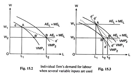
In this article we will discuss about the individual firm’s demand curve for labour when several variable inputs are used.

The MPT gives us an individual firm’s labour demand curve (under perfect competition) when only one variable input is used—this curve slopes downwards to the right. We shall now assume that the firm uses more than one variable input.

This assumption is more realistic than the single variable input assumption. Let us assume that the firm uses labour along with some other variable inputs. We have to derive the firm’s labour demand curve in these conditions.

Let us state, to begin with, that here a single MRP_L = VMP_L curve of the firm would not be its labour demand curve. This is because, in this multiple variable input case, a change in the price of labour causes a change in the quantities used of the other variable inputs, which, in its turn, would affect the MP_L, and cause a shift in the MP_L curve.

A ceteris paribus change in W would have three effects upon the use of labour and upon the uses of the other variable inputs. These effects are known as the substitution effect (SE), the output effect (OE) and the profit maximising effect (PME).

Let us suppose that in Fig. 15.2, initially the firm is in equilibrium at W = W₁, at the point A on the VMP, curve, which is the point of intersection between its MRP_L = VMP_L (viz., VMP₁) curve and the ME_L curve.

At point A, the firm is buying L₁ of labour at the wage rate W = W₁, Let us suppose now that W falls from W₁ to W₂. As a consequence of this, the firm’s VMP_L curve would shift rightwards from VMP₁ to VMP₂. We may explain this shift in the following way.

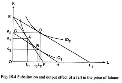
Let us refer to Fig. 15.4 where we have assumed that the firm uses only two variable inputs, labour and capital. Initially, with W = W₁ and a given price of capital, the firm’s iso-cost line (ICL) is, say, EF and the firm is in equilibrium at the point A, where the ICL has touched one of its IQs, viz, IQ₁. At the point A, the firm uses L₁ of labour with of capital.

Let us now suppose that W falls, the price of K remaining constant and the firm’s expenditure remaining unchanged. As a result, the firm’s ICL would rotate from EF to EF₁—the ICL would now become flatter because the ratio of the prices of L and K has fallen. In Fig. 15.4, the firm’s equilibrium point would now move from the point A to the point C on a higher IQ₁ viz., IQ₂.

The firm now buys more of both the inputs and produces a higher level of output. This effect may be called the total effect (TE) of the fall in W. This TE can be broken up into a substitution effect (SE) and an output-effect (OE).

The Substitution Effect:

The SE is the effect of a change in the relative prices of the inputs, the firm producing the same quantity of output. First, we have to obtain this effect (i.e., SE). With the fall in W, the price of K (r_K) remaining constant, relative prices of the inputs have changed. If, now, the firm has to produce the same quantity of output, its expenditure would fall.

So, let us curtail its expenditure accordingly. As a result, its ICL would have a parallel leftward shift from EF₁ to GH, the latter being a tangent to IQ₁ at the point B.

In other words, if W falls from W₁ to W₂, r_K remaining constant, causing a change in the relative prices and if the firm has to produce the same quantity of output as at A, then its equilibrium point would have to move from A to B along IQ1.

At the point B, the firm would use more of labour, viz., L = L₃ and less of capital, viz., K = K₃—it would substitute labour, which has become relatively cheaper, for capital, which has become relatively dearer. This is the SE of the said change in W.

The Output Effect:

We may now obtain the output effect (OE). In order to obtain the SE, we had curtailed the firm’s expenditure. Let us now restore the expenditure to its original level. The firm’s ICL, viz., GH, will have a parallel rightward shift from GH to EF₁, and the firm’s equi­librium point (the point of tangency) would move from B on IQ₁, to C on a higher IQ, IQ₂, raising the firm’s output to a higher level.

That is, if W falls, r_K and the expenditure remaining constant, firm’s output would increase. This is the output effect of the said fall in W. This effect is represented by the movement of the firm’s equilibrium point from B to C. In Fig. 15.4, owing to the output effect, the firm would be increasing its use of both the inputs (unless any of them is an inferior input).

Shift in the VMP_L Curve:

What we have obtained, then, is this. The SE of a fall in W would cause a substitution of labour for capital. Owing to this effect, the MP_L curve would shift to the left, for, now there is less of capital to work with. But the total effect (SE + OE) of the said fall in W would generally result in increasing the use of both the inputs.

In Fig. 15.4, if we compare the points A and C, we find that as a result of a ceteris paribus fall in W, the firm uses more of capital along with an increased use of labour. Since labour now has more of capital to work with, the total effect of a fall in W would cause the MP_L curve and, therefore, the MRP_L = VMP_L curve, to shift to the right.

It may be noted, however, that the output effect alone may cause the MP_U curve to shift to the right. In Fig. 15.4, owing to the output effect, use of labour has increased by L₃L₂ and the use of capital has increased by K₃K₂ which is larger than the SE fall in the use of capital by K₁K₃.

Derivation of the Demand Curve for Labour:

We may now come back to Fig. 15.2 to see that as W falls from W₁ to W₂, the MRP_L = VMP_L curve of the firm shifts to the right from VMP, to VMP₂. Therefore, at W = W₂, the firm would be in equilibrium at the point B on the VMP₂ curve and not at the point B’ on the VMP₁ curve. The equilibrium point, B at W = W₂, is the point of intersection between the MRP_L = VMP_L curve of the firm which is VMP₂ and its ME_L curve.

We have obtained, therefore, that at W = W, the firm’s equilibrium labour-demand point is A and it buys L₁ of L and at W = W₂, that point is B and the firm buys L₂ of L. So, in more than one variable input case, the firm’s labour demand curve would be obtained if we join the points like Aon VMP] curve and B on VMP₂ curve, etc.

In Fig. 15.2 this curve is dd’, which would, of course, be sloping downward towards right giving us the usual inverse relation between the rate of wage and demand for labour.

We may conclude, therefore, that in a perfectly competitive labour market when the firm uses more than one variable input, its labour demand curve is not obtained as a particular segment of a single MRP_L = VMP_L curve. The labour demand curve would be made up of the points like A and B in Fig. 15.2 on the shifting VMPP_L curves.

We shall end our discussion of the topic by mentioning one final point. In Fig. 15.2, we have assumed that, as W falls, by any amount whatsoever, the MP_L curve, and, therefore, the MRP_L = VMP_L curve shifts to the right, i.e., as W falls, the MRP_L = VMP_L curve shifts uniformly to the right. But this may not happen always.

Everything depends on how the quantity used of capital (in the two-input, L and K, case) responds to a fall in W. It may so happen, therefore, that the MP_L curve and so MRP_L = VMPP_L curve shifts uniformly to the left as W falls, for example, from VMP₁ to VMP₂ curve in Fig. 15.3.

We may also obtain that as W falls, the VMP_L curve shifts from VMP₁ in Fig. 15.3 to a twisted VMP₂ curve—some part of the latter lying to the left and some part lying to right of the former curve.

In either case, as W falls, use of labour rises—from L₁ to L₂ or L’₂, i.e., in either case, the labour demand curve slopes downwards to the right—passing through points like A and B or through A and B’. The labour demand curves in these two cases have been obtained in Fig. 15.3 to be d’d’ and d”d”, respectively.

The Profit Maximising Effect:

We have said that a change in W would have three effects. Two of them, viz., SE and OE. However, we have not yet discussed the third effect, viz., the profit- maximising effect (PME).

For, we have seen the second effect, viz., the output effect (OE) was alone sufficient to cause a shift in the firm’s MP_L and MRP_L = VMP_L curve. We shall now see that the PME also normally causes an increase in the use of both the inputs (L and K). We shall now discuss the PME.

First, let us suppose that in Fig. 15.4, the initial output-maximising and profit-maximising equilibrium point of the firm is A. After a ceteris paribus fall in W, the new output-maximising equilibrium—subject to a given expenditure—is obtained at point C.

The input combination (L₂, K₂) at point C is, generally, not the profit-maximising combination. As W falls, the firm’s marginal cost curve (the upward sloping portion) shifts to the right reflecting a fall in MC at each output (unless labour is an inferior input).

As the MC curve shifts to the right, the firm’s profit-maximising output at the given price increases. In order to produce a larger quantity of output, the firm would have to increase its expenditure and move out along its expansion path to a point to the right of the point C, normally increasing both L and K. There­fore, the PME also causes the MP_L curve to shift to the right.