Shapes of TR, AR and MR Curves (With Diagrams)

Let us learn about the shapes of TR, AR and MR curves under perfect and imperfect competition.

Shape of TR Curve under Perfect and Imperfect Competition:

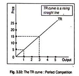
A firm, under perfect competition, behaves as a ‘price-taker’ in the sense that no single firm can influence the price of the product. Under this situation, the TR curve is a rising straight line from the origin. TR rises in direct proportion to output. The TR curve has been drawn in Fig. 3.32 whose slope is the given price in the market.

In any branch of imperfect competition (say, monopoly or monopolistic competition or oligopoly), a firm behaves as the ‘price- maker’ in the sense that it can influence the price of the product. A firm has to reduce the price of the product if it wants to sell more. So TR must rise.

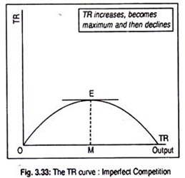
However, TR does not increase in proportion to the increase in the volume of sales. Under imperfect competition, TR initially rises, reaches maximum when OM units of output are sold, and then starts declining as output sold increases over time.

This shape of the TR curve has been shown in Fig. 3.33:

Shapes of AR Curve under Perfect and Imperfect Competition:

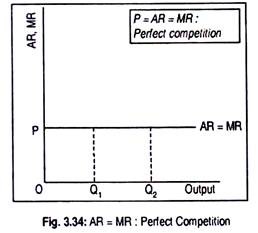
As a competi­tive firm behaves as a price-taker, its AR remains the same even if volume of sales increases. That is why the AR curve of Fig. 3.34 has been drawn parallel to the horizontal axis. AR curve shows that, at price OP, any amount of the goods (OQ₁ or OQ₂) may be demanded. In other words, the AR curve or the demand curve faced by a competitive firm becomes perfectly elastic.

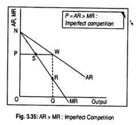
Under imperfect competition, AR curve becomes negative sloping. It declines continuously as price declines. However, demand curve of a monopolistically compe­titive firm is more elastic than that of the demand curve faced by a competitive firm.

In Fig. 3.35 linear AR and MR curves have been drawn. They can be non-linear also.

Shapes of MR Curve under Perfect and Imperfect Competition:

Under any market situation, AR is the same as the price. As price is given, MR is equal to the given price, i.e., AR = MR.

This can be shown in the following way:

We know that TR = P × Q

AR = TR/Q = P × Q/Q = P

MR = ∆TR/∆Q

Under perfect competition, as price does not change, TR changes only in proportion to the change in the volume of sales.

Thus,

MR = P × ∆Q/∆Q = P

.^.. AR = MR

That is why AR curve is identical to the MR curve under perfect competition, as shown in Fig. 3.34.

On the other hand, as a firm under imperfect competition can change the price of the product, AR no longer coincides with MR. Here

TR = P × Q

AR = TR/Q = P

MR = ∆TR/∆Q = ∆P × ∆Q/∆Q = ∆P

.^.. AR > MR (^._.^. P > ∆P)

That is why AR curve has been drawn above the MR curve in Fig. 3.35.

At OQ output level, AR = QW and MR = QR. Thus TR in accordance with AR is

TR = P.Q = OP.OQ = OPWQ

and TR, in accordance with the MR, is

TR = OP.OQ = ONSRQ.

Thus, OPWQ = ONSRRQ. Note that in the measurement of TR we have OPSRQ area. Thus, A PNS = A SWR. This means PN = WR.

Therefore, AR = WQ = 2MR = 2(RQ) or MR = ½ AR. This means that the slope of MR is twice the slope of AR. Geometrically, MR curve falls twice as fast as the AR curve.

If the AR curve is a linear one, the MR curve must bisect the horizontal distance between the AR curve and the vertical axis. Further, as the AR curve is downward sloping, so is the MR curve.

One thing should be remembered regarding TR and MR relationship. MR is the slope of TR. When TR rises as output rises, MR declines. When TR reaches maximum, MR becomes zero and, when TR declines, MR becomes negative.