Joint Demand and Supply (With Diagram)

The below mentioned article provides an overview on Joint Demand and Supply. After reading this article you will learn about: 1. Meaning of Joint Demand 2. Meaning of Joint Supply.

Meaning of Joint Demand:

Joint demand refers to the relationship between two or more commodities or services when they are demanded together. There is joint demand for cars and petrol, pens and ink, tea and sugar, etc. Jointly demanded goods are complementary.

A rise in the price of one leads to a fall in the demand for the other and vice versa. For example, a rise in the price of cars will bring a fall in their demand together with the demand for petrol and lower its price, if the supply of petrol remains unchanged.

On the contrary, a fall in the price of cars, as a result of a fall in the cost of production of cars, will increase their demand, and therefore increase the demand for petrol and raise its price, if available supplies of petrol are unchanged.

Figure 1 (A) illustrates the market for cars and Figure 1 (B) for petrol. When the price of cars increases from OP to OP₁ their demand is reduced from OQ to OQ₁ .The demand for petrol falls, as shown by the dotted curve D₁ in Panel (B) whereby the quantity demanded falls from OQ to OQ₁ As a result, the price of petrol also falls from OP to OP₁ .

Thus the prices of jointly demanded goods tend to move in opposite directions, depending upon the degree of elasticity of demand for cars and the supply of petrol.

If, however, the demand for one product (cars) falls from D to D₁ in Figure 2 (A), the demand for the other product (petrol) will also decline from D to D₁ in Panel (B) of the figure. As a result, the prices of both the products will fall from OP₁ to OP. On the contrary, an increase in the demand for one product (cars) will raise the demand for the other product (petrol), and consequently the prices of both will rise.

Figure 2 (A) illustrates the case of a fall in the demand for cars from OQ to OQ₁ with the consequent fall in the demand for petrol from OQ to OQ₁ as shown in Panel (B). Both the figures also depict fall in the prices of the cars and petrol from OP to OP₁. The extent to which these prices will change depends upon the degree of elasticity of demand for the products combined with the degree of scarcity or abundance.

But what are the forces which lie behind the demand and supply schedules of jointly demanded products’? It is possible to know the marginal cost of production of the commodities demanded jointly, but difficult to estimate their separate demand schedules.

The marginal analysis helps to solve the latter problem. In order to calculate the marginal utility of one product, we take two separate combinations of the two products in which the quantity of one product is used in different proportions while of the other is kept constant.

“We can take the various possible combinations of the factors of production, and contract two cases in which different quantities of one factor are employed together with equal quantities of others. The extra product which will be yielded in the case in which the larger quantity of the varying factor is employed, can then be regarded as the marginal product (or marginal utility) of the extra quantity of that factor. We can say that the employment of this factor will be pushed forward to the point where this marginal product will be roughly equal to the price that must be paid for it.”

We illustrate with the aid of an example the case of the jointly demanded goods, pen and ink:

1 Pen + 1 Inkpot = Rs.4.00 worth of utility

2 Pens + 1 Inkpot = Rs.6.50 worth of utility.

Therefore, the utility of an additional (marginal) unit of one pen equals Rs. 2.50. Thus the marginal utility of one pen equals Rs. 2.50. Similarly, the marginal utility of ink can be calculated by varying the quantity of ink and keeping the quantity of pen constant.

Thus price will settle at a point where the marginal utility of a product equals its marginal cost of production and the price or demand of one product will affect that of the other in the manner illustrated in Figures 1 and 2.

In a similar manner, it is possible to estimate the separate marginal product of each factor of production demanded jointly. For the building of houses, building materials like cement, bricks, steel, timber and labour are jointly demanded, and the marginal productivity of each can be calculated by varying one factor and keeping all others constant.

Derived Demand:

The case of joint demand for producers’ goods is referred to as derived demand because the demand for any factor is a demand derived from the final product which that factor helps to produce. The demand for labour is a derived demand. It depends on the demand for the product it helps to make.

The demand for masons, unskilled labourers, carpenters and plumbers is derived from the demand for houses, though all are jointly demanded. An increase or decrease in the demand for houses raises or lowers the demand for such labour needed for house building. The demand price of the house-building labour is derived from the demand price of houses.

Marshall conceived of certain conditions when a particular factor (say, masons) demanded jointly with other factors can raise its remuneration by withholding its supply. Suppose the masons employed for building houses threaten to withhold their supply if their wages are not raised.

According to Marshall, workers who are jointly demanded with other factors would be successful in raising their wages if:

(i) The demand for the services of that set of workers is inelastic;

(ii) The demand for the commodity which the group of workers helps to produce is inelastic;

(iii) The wage bill of this group forms a very small proportion of the total wage bill so that, a rise in their wages does not substantially affect the total cost of production of the commodity; or

(iv) If the other cooperate factors are squeezable, i.e., the wages of the other workers are reducible or the suppliers of other factors are forced to accept low prices.

Thus a factor of production will be successful in raising its remuneration if any of these conditions are fulfilled.

Meaning of Joint Supply:

There are a number of products which have a common source of supply in that they are produced jointly. The production of one automatically involves the production of another, such as wool and mutton, wheat and straw, cotton and cotton seed, etc. Joint products are also known as joint cost products.

Joint products are of two types: first, whose proportions cannot be varied; and second, whose proportions can be varied. Products like wheat and straw, or cotton and cotton seed fall in the first category. If there is bumper wheat or cotton crop, the supply of straw or cotton seed is automatically increased. But it is difficult to separate the cost of production of such products.

However, the price of each product can be fixed on the principle of ‘what the traffic will bear’ that is, what the product will fetch in the market. In other words, the price of each product will be determined by the marginal utility of each product to consumers. But the price of each product must be such that the sum of the revenues from their sale must equal their total cost of production.

Joint Products with Fixed Proportions:

In the case of such joint products whose proportions are fixed by nature, if the demand for the major product, say wheat, increases, its price would rise. This would encourage its production which will also increase the supply of its minor product, say straw. As a result, the price of the minor product (straw) would fall. This is illustrated in Figure 3 (A) and (B).

Figure 3 (A) depicts the case of wheat, and Figure 3 (B) that of straw. When the demand for wheat increases from D to D₁ the price of wheat rises from OP to OP₁ and the quantity of wheat increases from OQ to OQ₁ .This leads to the increase in the supply of straw from OQ to OQ₁ (shown by the shifting of the curve S to the right as S₁,). As a result, the price of straw falls from OP to OP₁

Joint Products with Varied Proportions:

In the second category fall such joint products as wool and mutton whose proportions can be varied. In the case of such products price can be determined by varying the proportions of the products. For example, sheep yield wool and mutton, but their proportions vary from breed to breed.

By judicious cross-breeding of sheep, farmers can rear sheep that will yield more wool than mutton, or more mutton than wool, according to their requirements.

Suppose an Australian farmer wants to have more wool than mutton. He finds that a certain number of sheep of a particular breed yields a given quantity of wool and mutton, and that a large number of sheep of another breed yields more wool and less mutton. He obtains the surplus wool by the extra expenditure of rearing the additional number of sheep. The extra cost of grazing is the marginal cost of wool.

In a similar way, he can ascertain the marginal cost of mutton, if he requires more mutton than wool. The price of each product will thus be determined by the equality of the marginal cost and the marginal utility of each product taken separately. Let us take a numerical example to explain the pricing phenomenon of joint products.

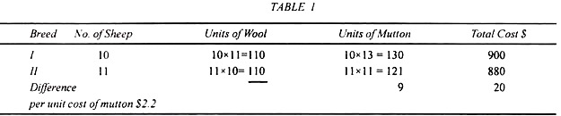
Suppose it costs an Australian farmer $ 90 each to rear a breed of sheep that yields 11 units of wool and 13 units of mutton, while another breed costs $ 80 each and yields 10 units of wool and 11 units of mutton. If he breeds 10 sheep of the first type and 11 sheep of the second type, then the marginal cost of a unit of mutton would be $ 2.2, as shown in Table 1.

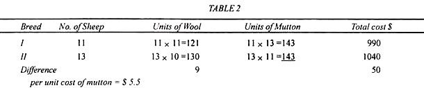
Now to calculate the per-unit cost of wool, suppose he breeds two other varieties of sheep which cost the same per sheep, i. e„ $ 90 and $ 80 each. He breeds 11 sheep of the first type and each sheep yields 11 units of wool and 13 units of mutton.

Similarly, he breeds 13 sheep of the second variety and each yield 10 units of wool and 11 units of mutton. In this case, the per unit marginal cost of wool would be $ 5.5, as shown below in Table 2.

The interrelationship of the prices of such joint products whose proportions are variable is depicted in Figure 4. S_w is the marginal cost (supply) curve of wool and S_M is the supply curve of mutton. Let D be the original demand curve for the two products. As a result, Q_w quantity of wool is sold at P_w price, and Q_m quantity of mutton is sold at P_m price.

Suppose the demand for wool rises, as shown by the upward shifting of the demand curve D to D_{1 .}It will raise the price of wool to P₁w and increase its supply to Q₁w. But the increase in the supply of wool as a result of the higher demand price would not lead to a proportional increase in the supply of mutton.

The percentage increase in the supply of mutton would depend entirely on the extent to which the proportions between the two could be varied.