Perfect Competition: 12 Things to Know about Perfect Competition

Everything you need to know about Perfect Competition.

Equilibrium for the firm under perfect competition can only occur when the marginal cost of the firm is rising at and near equilibrium output – A. Stonier and D.C. Hague.

Perfect Competition # 1. Subject Matter:

A market is said to be perfectly competitive when all firms act as price takers—when they can sell as much as they like at the going price but nothing at a higher price. This is because every firm is so small a part of the market that it can exert no influence on market price by selling a little more or little less of its product. This is usually observed in markets for agri­cultural commodities like jute, cotton, wheat, etc. The stock market is another example of this.

Perfect Competition #  2. Conditions:

A set of conditions that must be satisfied to guarantee this result is sometimes known as the assumptions of perfect competition.

These are:

(i) A Homogeneous Product:

A product which is the same for every firm in the industry is called a homogeneous product. One farmer’s carrots are indistin­guishable from those produced by any other farmer. They are homegeneous. By contrast, the Maruti Udyog’s Gypsy model is distinct from car models of all other motor manu­facturers, and from Maruti’s other models. The product is differentiated.

(ii) Many Sellers:

For firms to be price-takers, the number of sellers must be large enough so that no single firm acting by itself can exert any perceptible influence on the market price of its product by selling a little more or little less of the product. This is another key distinction between, for example, the car industry and the carrot industry. A single farmer’s contribution to the Total production of carrots is a very small portion of the total.

He could double his production, or produce some other crop with no large effect on the total market supply, and, therefore, the price of carrots. In contrast, Maruti Udyog’s car output is a signi­ficant part of total car production in India. The company does have the power to influence price by varying the number of cars it produces. Of course, the power is not unlimited (because there are other producers of cars), but it certainly exists.

(iii) Perfect Information:

When buyers of the product are fully informed about the prices and qualities of goods offered for sale by sellers, they are said to have perfect information. As a consequence, if any firm raises the price of its (homo­geneous) product above the prices charged by other producers, it is sure to lose all its customers. This is because people will not buy a commodity from a firm at one price if they know that the same product can be obtained at a lower price from another firm. Hence price prevails in all parts of the market.

(iv) Freedom of Entry and Exit:

Assumptions 1, 2 and 3 relate to individual firms. The fourth assumption relates to the whole industry. Freedom of entry means that a new firm is free to start production if it so
desires. There are no barriers to the entry of new firms in the industry. There are no legal or other restrictions on entry. Freedom of exit means that any existing firm is free to stop production and leave the industry if it so desires. There are no restrictions on exit, legal or otherwise.

Perfect Competition #  3. The Demand Curve for a Firm:

In order to develop a theory of commodity, pricing and output determination under pure competition, we have to derive, at the outset, the demand curve faced by the firm.

In pure competition, an individual firm produces a product which is the same as those of other firms. The firm is also so small a part of the market that it cannot exert any perceptible influence on market price. Hence, each perfectly competitive firm acts as a price-taker. It faces a price that is determined by market forces which are beyond its control. The firm’s problem is then, to decide whether to produce at all, and, if so, how much to produce in order to maximise profit.

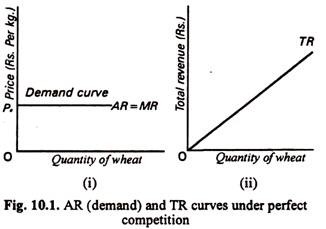
The demand (average revenue) curve for a price-taking firm is a horizontal straight line at the going market price. In Fig. 10.1(i) we show the demand curve for a firm under perfect competition. We initially assume that price has been determined at p₀ by the forces of supply and demand.

The firm can sell as much as it likes at the price p₀. If it raises its price above p₀ its sales will fall to zero, since all its customers realise that they can buy the identical product from other firms at price p₀. In other words the demand curve is completely elastic at price p₀.

A perfectly elastic demand curve has an important implication the average revenue from the sales of all units will be equal to the marginal revenue from the sale of an extra unit. Recall that average revenue is another word for the price at which the firm sells its product.

Marginal revenue is the change in total revenue associated with the sale of an additional unit of the product. Since the firm can sell as much or as little as it likes at the going price, marginal revenue is always equal to average revenue under perfect competition.

Consider, for example, a producer who faces a market price of 25 paise per kg for carrots. Since every kg of carrots he sells brings in 25 p average revenue per kg of carrots is 25 p. Also, since price is given at 25 p each additional kg sold will bring in 25 p, i.e., marginal revenue is also 25 p. So the important point to note is that: MR = AR for the firm under perfect competition.

The demand curve faced by the firm is, thus, the same as both the average and the marginal revenue curves. All three coincide in the same straight line as in Fig. 10.1 (i), showing that p = AR = MR. For an industrial producer, all are constant regardless of the quantity of carrots he offers for sale. However, the producer’s total revenue is not constant at all levels of output (sales). Since price is constant, total revenue increases in direct proportion to output, as shown in Fig. 10.1(ii).

Thus in this context, we may note that there are two demand curves in perfect competition — a downward sloping market demand curve (which is the sum-total of the demand curves of different consumers) and the demand curve of an individual seller (which is horizontal). The market price is determined by the forces of demand and supply. And a price-taking firm can sell as much as it likes at the going price — its demand curve is completely elastic. Hence MR = AR = P. [Since MR = P (1 – 1/e_p) and e_p → ∞, 1 / e_p = 0. Therefore MR = P.]

Perfect Competition #  4. Equilibrium of a Firm under Perfect Competition:

These curves have no relation to market structure and are, therefore, universally applicable. We have just examined the nature of revenue curve of a firm in perfect competition. Now we can put the two sets of curves together and apply the two rules of profit-maximisation to find out the optimum output of a firm.

Perfect Competition #  5. Application of the MR-MC Rule:

If a competitive firm has to produce any­thing at all, it must choose that level of output for which MC = MR, Since MR = P, here this rule may also be expressed as MC = P.

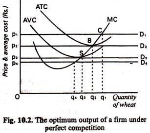
The profit-maximising rule is illustrated in Fig. 10.2. It shows the three cost curves of a firm as also four different demand curves the firm might face. If the demand curve is D₁, the firm can sell as much as it likes at the going price p₁. If the demand curve is D₂, it can sell any quantity at price p₂ and so on.

The MR-MC rule of profit maximisation tells us that when the demand curve is D₁. the optimum output is because this level of output corresponds to the point of intersection of the MC curve with the demand curve. If the demand curve is D₂, the equilibrium (or profit- maximisation level of) output is q₂ and so on.

Perfect Competition #  6. Application of Shut-down Rule:

Now we may apply the first rule of profit- maximisation to examine whether the firm should produce anything at all (under these four different demand conditions prevailing in the market) or close down its operation completely. When the demand curve is D₁ the firm is making excess (supernormal) profit because price is greater than average total cost. So the question of shutting down or closing down its operation does not arise. Now let us consider demand curve D₂.

This is tangent to ATC at point B. Now the firm is able to cover all costs and succeeds in making normal profit. Thus the level of output is Q₂ which enables the firm to equal P with MC. Thus, in this case also, the question of leaving the industry does not arise.

We may now consider demand curve D₃. It is tangent to AVC curve at point S. The corresponding output is q₃. At this point the firm is just able to cover its variable cost and is indifferent between staying in business and closing its operations. The firm is not earning enough to cover even a portion of its fixed cost.

Finally, when the demand curve is D₄, the firm can produce at best q₄ units output at a price p₄ if it is to stay in business. But when price is p₄ even varied cost cannot be covered, not to speak of fixed costs. Thus it would be worthwhile on the part of the firm to shut down or close down its operations completely. Hence its output in such a situation would be zero.

Perfect Competition #  7. Supply curve of a competitive firm:

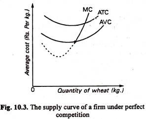
Now we may formally derive the supply curve of a competitive firm. It may be recalled that a firm’s supply curve shows the relation between the market price of the commodity and the desired output of the firm. We know by now that a profit-maximisation firm’s equilibrium level of output is reached when P = MC. In Fig. 10.3 we see that when the market price is p₄, its optimal output is low. When price rises to p₃ it produces a positive quantity of output q₃.

When price continues to rise to p₂ and p₁ its optimum output also increases to q₂ and q₁. Thus the minimum price acceptable to the firm to start production is p₃ which price is equal to AVC at point S. This is why the lowest point of the A VC curve is called the shut-down point of a firm under perfect competition. It also follows that, that portion of the MC curve which lies above the shut-down point S, is the supply curve of a competitive seller.

It may be noted the decision to produce one extra unit is governed by MR and MC. Thus when P = MR increases due to upward shift of the demand curve the competitive firm finds it profitable to produce more and it continues to move along the rising portion of MC curve.

The MC curve is upward sloping from left to right due to the operation of the law of diminishing return. This causes of MC curve to rise as output expands. The process continues until the inequality P = MR > MC is converted into an equality (P = MR = MC). Thus in Fig. 10.2 SBCMC is the supply curve. This is shown separately in Fig. 10.3.

The long-run supply curve can also be derived in the same way for the long-run marginal cost (LRMC) curve.

However, the firm enjoys more flexibility in the long-run for two reasons:

(a) all factors are variable and,

(b) the firm can choose among plants of different sizes because of the possibility of factor substitution and its ability to vary techniques of production.

It may be recalled that the LRMC is the cost of producing the extra unit of output by using the most efficient plant from those that are available in the long run.

Perfect Competition #  8. Supply curve of the industry:

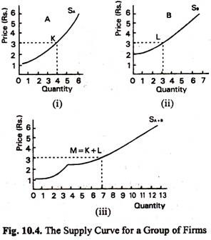
Figure 10.4 illustrates the derivation of an industry supply curve for an examination of only two firms.

The important point to note here is:

The supply curve for a competitive industry is just the horizontal sum of the marginal cost curves of all the individual firms belonging to the industry.

This supply curve, based as it is on the short-run marginal cost curves of the firms in the industry, is the industry’s short-run supply curve.

Figure 10.5 shows that, at a price of Rs. 3, firm A would supply 4 units and firm B would supply 3 units. Together, as shown in (iii), they would supply 7 units. In this example, because firm B does not enter the market at prices below Rs. 2, the supply curve S_A+B is identical to S_A up to price Rs. 2 and is the sum of S_A+ S_B above Rs. 2.

If there are hundred identical firms—all alike in size-efficiency and capital structure the industry supply curve would simply be a hundred-fold extension of the supply curve of an individual firm.

Perfect Competition #  9. Long-run Industry Equilibrium:

After examining the equilibrium of a firm we may discuss the nature of equilibrium of a competitive industry in the long run.

In order to show industry equilibrium under perfect competition we have to draw market supply and demand curves. The market demand curve is downward sloping because it is the sum of the demand curves of individual curves. Likewise the market (industry) supply is the sum of the marginal cost curves of the firm. This is derived by horizontally summing the supply curves of individual firms.

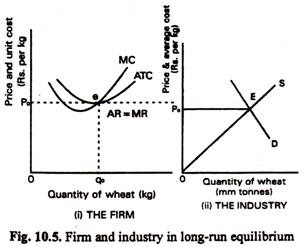
In Fig. 10.5 we have drawn the supply and demand curves in part (ii) and cost curves of a typical firm in part (i) This firm is one of many firms belonging to the industry and produces only an insignificant part of industry output. On the vertical axis we measure price. On the horizontal axis we measure output of wheat. The firm’s output is measured in kg and industry output in million tonnes.

Fig. 10.6 shows the position of an individual firm when the industry as a whole is in long- run equilibrium. In part (ii) we show that equilibrium price (p₀) is determined by the market forces, i.e., by the intersection of the market demand and supply curves. At this point the firm’s demand (AR) curve is completely elastic.

The firm reaches equili­brium at point e where MC = MR. Its equilibrium output is q₀ at that market price. Since P = ATC, P x Q = ATC x Q = TC. Thus, the firm is making enough revenue so as to cover all costs (fixed and variable) including normal profit. In the long run the firm must cover all costs in order to stay in business.

Entry and Exit of Firms:

The key to long- run industry equilibrium in a competitive market is entry and exit. When P = ATC and TR = TC a firm is said to be breaking even. This is why the lowest point of the ATC curve is called the break-even point. When all firms in a competitive market reach their respective break-even points, the industry is said to be in equilibrium.

In other words, when firms are just breaking even, they are covering all costs (including the opportunity cost of capital). Thus, there is no reason why they should leave the industry. Again since no excess profit is being made by any firm, there is no incentive for any new firm to join the industry either.

Thus, there is unlikely to any change in the level of output of any of the member firms. In other words, the industry has reached long-run equilibrium. However, if existing firms make excess profit, new firms will be tempted to join the industry. By contrast, if some firms incur losses due to internal inefficiency they will leave the industry. It is because a better return can be obtained by employing capital elsewhere.

Perfect Competition #  10. Long-run Disequilibrium:

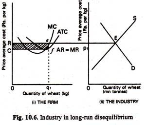
We may now show two disequilibrium situations under perfect competition. In Fig. 10.6 the market price is p₁ in part (i). This is greater than the ATC of the firm shown in part (i). So the firm is making excess profit of ef per unit. The shaded area of p₁efc shows total excess profit, i.e., the difference between TR and TC. So the industry is in a disequilibrium situation. The excess profit will now attract new firms into the industry. New entry will cease only when the excess profit has been virtually shared by new firms and wiped out subsequently.

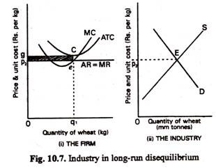
An exactly opposite type of situation is shown in Fig. 10.8. Here the market price p₂ is less than ATC of the firm under consideration. Thus there is loss of ce per unit or a total loss of p₂gce — the shaded area of Fig. 10.8. This will cause some of the firms to leave the industry.

The process will continue until and unless the losses are wiped out. Thus the zero profit long-run equilibrium is a tangency solution in any case. No firm can make excess profit nor incur losses in this type of market in the long run.

Perfect Competition #  11. Shifts of the Supply Curve in the Long-Run:

The entry and exit of firm provides two basic mechanisms through which a competitive industry reaches its long-run equilibrium in the presence of super-normal profits or losses. However, if only one or two firms enter or leave the industry, total supply is likely to remain unchanged. However, the entry or exit of a large number of firms at the same time in a disequilibrium situation will change the market price. Let us see how this happens.

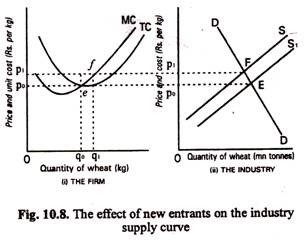
The market price will be altered if there is a shift of the supply curve. Recall that the short-run supply curve is the sum of the MC curves of those firms that are in the industry at present. If new firms join the industry due to the presence of super-normal profits, the industry’s supply curve will shift to the right from S to S¹ as is shown in Fig. 10.8. It is because new firms will add to existing industry output.

Consequently market price will fall from p₁ to p₀. So the demand curve faced by the firm [shown in 10.8(i)] will shift down­ward. The market share of the firm will fall (as is shown by a fall in equilibrium output from q₁ to q₀). Thus both old and new firms will make output adjustments in this new price.

The new MC-MR equality of the old firm occurs at e. New firms continue to join the industry as long as excess profits can be made. With every new entry the supply curve shifts to the right. If there are substantial new entrants into the industry, the supply curve eventually shifts to S¹ so as to cause market price to fall to the old level and excess profit to disappear.

The industry again reaches long- run equilibrium since each firm reaches its break-even point (as in Fig. 10.5). [One can also show the exit of firms continues until a new long-run equilibrium is reached. This is left as an exercise to the student.]

Perfect Competition #  12. An Alternative Analysis Using TR and TC Curves:

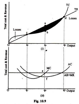
Our analysis of the firm under perfect com­petition has so long been based on average and marginal cost and revenue curves. However, it is possible to find out the same profit- maximising level of output by using total revenue and total cost curves. For the sake of simplicity we restrict out-selves to the long- run situation. Since in the long run all costs are variable the long-run total cost curve starts from the origin. Such a curve is shown in Fig. 10.9.

The equilibrium position of the firm is illustrated in Fig. 10.9. Since under perfect competition price remains constant at all levels of output, the TR curve is a straight line with unchanged slope (as is given by the ratio c/q, c/q₀, or d/q₂). Since the slope is constant, MR is constant and when MR is constant it is equal to AR.

The firm maximizes profit by making the difference between TR and TC as large as possible. This happens when the firm produces q₀ units of output per period. At this level of output MC is also equal to MR (and the MC curve intersects the MR curve from below, as is indicated by point e).

Total Revenue and Cost curves for a firm under perfect competition. Optimum output is where the vertical difference between TR and TC is maximum at output q₀, where the firm makes super-normal profits (a – b). This corresponds to output where MC = MR. Losses occur at outputs below q₁ and above q₂.

In Fig. 10.9 q₀ is the equilibrium output for the firm. What about the industry to which the firm belongs? We have to recall that the industry reaches equilibrium when there is neither entry of new firms into or exit of old firms from the industry.

This happens when each firm makes just normal (or zero excess) profits, neither more, nor less. But in Fig. 10.9 we see that the firm under consideration is making excess profit (as measured by the vertical distance of a – b). This will induce new firms to join the industry.