Determination of Equilibrium Prices (With Diagram)

Let us examine how equilibrium prices are determined in different time periods:

A. Market Period Price Determination:

In order to determine prices under market period, Dr. Marshall divided commodities into two categories:

1. Perishable Goods

2. Durable Goods

1. Perishable Goods:

Perishable goods refer to those goods which perish very quickly. In simple terms, goods which cannot be stored for some time are called the perishable goods. Fresh vegetables, milk etc. are included in this category. Supply of such goods at any given time is fixed. If demand increases supply cannot be increased so quickly. Therefore, it is demand that plays a dominant role in the determination of price.

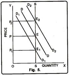
In figure 5 quantities of perishable goods is measured on horizontal axis, price on vertical axis. SS is the supply curve. It signifies the fact that supply of perishable goods remains fixed. DD is the original demand curve which shows the equilibrium at paint E. Thus, OP is the equilibrium price. Now, suppose, if in the very short period demand increases and assumes the form of D₂D₂.

The equilibrium will also shift to E₂. It depicts that with the increase in demand the price increases to OP₂. On the contrary, if the demand falls from DD to D₁D₁, the equilibrium will shift to E₁ from E side by side price will fall from OP to OP₁.

2. Durable Goods:

Durable goods are those which can be reproduced or those can be stored. Like perishable goods, the supply of durable goods is not vertical throughout the length. Firms selling such goods have a minimum reserve price. They will not sell goods at less than the reserve price. These goods are like wheat, soap, oil etc.

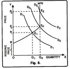
MPS is the market period supply curve where OQ₀ is the stock of the commodity. To start with the demand for the commodity is shown by D₁D₁ where the price is OP₁ and quantity supplied is OQ₁. Q₁O₀ stock will be held back. If the demand is D₂D₂, the whole stock will be sold out at OP₀ price. But in case the demand is D₂D₂, the equilibrium will be at E₂ and the price will be OP₂ where the entire output is sold.

At OR price i.e. ‘the ‘Reserve Price’ the entire output is held back. But from R to Eo, as the price rises, the quantity supplied also rises.

Factors Affecting Reserve Price:

Following are the factors which go a long way to affect the reserve price:

1. Price in Future:

If the seller expects that a high price will prevail in the market in future, the reserve price will be higher and vice-versa.

2. Liquidity Preference:

If the seller is in urgent need of money, his reserve price will be lower. Thus, higher the liquidity preference, higher will be the reserved price and vice-versa.

3. Future Cost of Production:

If the seller expects that in future the cost of production will fall, his reserve price will be lower and vice-versa.

4. Storage Expenses:

If the seller finds that the storage expenses are higher and the time for which the stocks have to be held are longer, his reserve price will be lower and vice-versa.

5. Durability of Commodity:

The durability of the commodity influences the reserve price. The more durable a commodity is, the higher will be the reserved price.

6. Future Demand:

The future demand of the commodity also influences the reserve price of the producer. If the producer expects a higher demand in future, his reserve price will also be higher.

B. Short Period Price Determination:

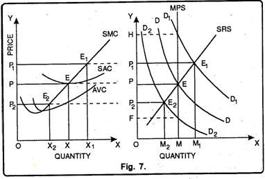
Price determination in the short period has been explained with the help of Fig. 7.

The figure 7 depicts the process of price determination in the short period. DD is the demand curve of the industry. MPS is the market period supply curve while SRS is the short run supply curve of the industry.

Initially, OP is both the market price as well as the short run price. At price OP the individual firm will adjust its output OX. At equilibrium level of output OX, price is equal to its marginal cost and marginal cost curve cuts the MR curve from below.

The firm enjoys normal profits. Now, suppose demand increases from DD to D₁D₁ and the industry is in equilibrium at point E₁ which determines the price OP₁ The new price OP₁ is less than the new market price i.e., OH. The reason is being that in the short run marginal cost curve rises as more is produced. Thus, the individual firm will take price OP₁ and will produce OX₁ level of output at which price OP₁ equals the marginal cost and the firm enjoys supernormal profits.

On the other hand, if the demand curve falls to D₂D₂ the new equilibrium will be established at E₂ and the price will falls to OP₂. But in the short period the firm will contract output by reducing the employment of labour and other variable factors Therefore, the new equilibrium level established at E₂ will determine the price OP₂ and the firms will produce OX₂ level of output. But, it is worth mentioning here that price OP₂ does not cover the SAC and the firms operating in the industry incur losses.

C. Determination of Long Period Normal Price:

Normal price comes to prevail in the long period. It is also called long period price. Normal price is influenced more by supply than demand. According to Marshall, “Normal price is that price which tends to prevail in a market when full time is given to the forces of demand and supply to adjust themselves”. Thus, it is clear from the definition that normal price is one that tends to prevail in the long period. It is not a real price.

Under perfect competition, the long run supply gets sufficient period to adjust itself to the changed conditions in demand. If supply is less than demand, price will rise. Thus, total supply will increase and all the producers will get normal profits only.

If supply is more than demand, price will fall and producers suffer losses. Some of the producers may leave the industry under pain of loss. Thus, total supply will decrease and once again price will rise to its normal level.

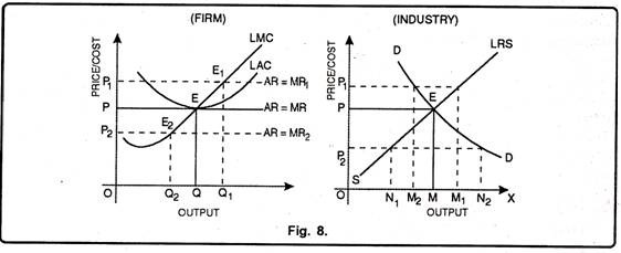
This has been illustrated with the help of figure 8 below:

In figure 8, we have taken output on X-axis and price on Y-axis. Industry’s demand curve DD and long run supply curve LRS cut at point E which determines OP price and OM output. If price by the industry is raised to OP₁, the demand is OM₂ and supply is OM₁ Since D < S, price will fall to OP On the other hand, if price is OP₂, in this case S < D. It is because at OP₂ price, supply is ON₁ and demand is ON₂. This will raise price to OP.

A firm under perfect competition in the long run is in equilibrium at output where Price = MC = Minimum LAC. This point is shown by E. It shows that the firm is making just normal profits. If the price is above the minimum long run average cost, the firms will be making super-normal profits.

In the diagram if the price is OP₁, in that case the firm will be producing OQ₁ output and would be making super normal profits. These super-normal profits will lure the new firms to enter the industry. With this, the supply of the industry would increase which would reduce the price and hence the existing firms will be left only with normal profits.

Q₁ the other hand, if the price is OP₂, in that case the firms will be in equilibrium at E₂ and hence the firm would be producing OQ₂. In this case the firm will be sustaining losses as AR < AC. Due to these losses, some of the firms will exit from the industry. This will reduce the supply which in turn would raise the price and hence the existing firms will be left with normal profits only.