
In this article we will discuss about:- 1. Conditions for Maximum Output Subject to a Cost Constraint 2. Conditions for Minimum Cost Subject to an Output Constraint.
Conditions for Maximum Output Subject to a Cost Constraint:
Let us suppose that the production function of the firm is:
q = f(x, y) [eqn. (8.21)]
where q is the quantity of output produced per period and x and y are the quantities of the two variable inputs used per period by the firm. It is assumed here that the first-order and second- order partial derivatives of q w.r.t. x and y exist.
ADVERTISEMENTS:
Let us also suppose that the cost constraint of the firm is given to be:
C° = rXx + rYy (8.38)
where C° is the fixed amount of money to be spent on the two inputs, and r1 and r2 are the prices of the two inputs, respectively. We intend to derive here the conditions for the output-maximising equilibrium of the firm subject to the cost constraint.
With a view to doing this, we would form the Lagrange function:
ADVERTISEMENTS:
V = f (x, y) + λ, (C° – rXx – rYy) (8.39)
where λ is the undetermined Lagrange multiplier.
Here V is a function of x, y and λ, and the first-order conditions (FOCs) for constrained output maximisation would be obtained if we set the first-order partial derivatives of V w.r.t. x, y and X equal to zero.
Therefore, the FOCs are:
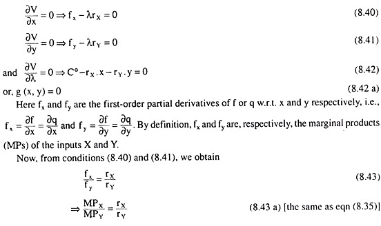

We have already known that (8.43) – (8.46) are the different forms of the FOC for constrained output maximisation and we have explained their economic significance. Let us note here two more things. First, equation (8.42) ensures that the cost constraint is satisfied.
Second, from (8.40) and (8.41) we have:
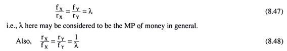
i.e., the reciprocal of X gives us the marginal cost of output in whatever way the firm increases its output—by using more of input X or more of input Y. We may now come to the second-order condition (SOC) of output maximisation.
The SOC gives us that the bordered Hessian determinant (D) should be greater than zero at the point of tangency where the FOC has been satisfied:
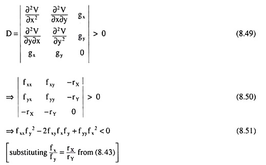
To understand the significance of the SOC as given by (8.43), let us remember the following:
The derivative of the slope of the isoquant is

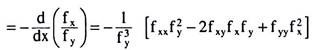
= positive (at the point of tangency where the FOC has been satisfied), due to the SOC (8.51) and since fy > 0 by the assumption of the MPS of the inputs being positive. Therefore, we have seen that the SOC implies that the derivative of the slope of the IQ would be positive, i.e., the IQ would be convex to the origin, at the point of tangency.
Since any point on an IQ may be point of tangency depending upon the slope of the iso-cost line, the SOC actually implies that the IQ should be convex to the origin throughout its relevant negatively sloped range where MPX, MPY > 0.
It may be noted here that, since the second-order or the sufficient condition (8.51) for constrained output maximisation is satisfied at each point within the domain of a regular strictly quasi-concave function, the production function (8.21) of the firm should be a regular strictly quasi-concave function. Only then the second-order condition would be satisfied.
ADVERTISEMENTS:
Incidentally, we may note that the conditions (8.43)-(8.46) are also the FOCs of the minimisation of output subject to a cost constraint. That is, output may be minimum also at the point of tangency between the ICL and an IQ.
However, in that case the SOC would be:
![]()
The significance of condition (8.52) is that the derivative of the slope of the IQ would be negative at the point of tangency, i.e., the IQ would be concave to the origin. That is, if the IQs of the firm are concave, not convex, to the origin, then at the point of IQ-ICL tangency, output would be minimum, and not maximum.
Conditions for Minimum Cost Subject to an Output Constraint:
ADVERTISEMENTS:
We shall now derive the conditions for minimising the cost of a particular amount of output. Let us suppose that the firm has decided to produce a particular amount, q°, of its output. Therefore, the firm would have to remain on a particular isoquant which is
q° = f (x, y) (8.53)
Let us also suppose that the cost equation of the firm is
C = rXx + rYy (8.54)
Here the Lagrange function relevant for constrained cost minimisation is
Z = rXx + rYy + μ[q° – f (x, y)] (8.55)
ADVERTISEMENTS:
where μ is the Lagrange multiplier.
Now, according to the Lagrange method, the FOCs for the constrained cost minimisation would be

Or, h (x,y) = 0 (8.58a)
Condition (5.58) ensures that the constraint on output is satisfied.
Again, from (8.56) and (8.57), we obtain:

What we have obtained here is that the FOCs of output maximization are the same as those of cost minimization.
Let us now come to the second-order or sufficient condition for constrained cost minimization which is given as the relevant borderd Hessian determinant being less than zero;

Since the condition (8.63) is the same as the condition (8.51), the SOC for cost minimisation is identical with that for output maximisation.