Top 11 Examples to Illustrate the Theory of Production

List of top eleven examples to illustrate the theory of production.

Example 1.

Suppose that a product requires two inputs for its production. Then is it correct to say that if the prices of the two inputs are equal, optimal behaviour on the part of the producer requires that these inputs be used in equal amounts?

Solution.

It is not correct to say that if the prices of the two inputs are equal, then these inputs should be used in equal amounts except in one case. We may explain as follows. Let us suppose that the production function of the firm is

q = f(x, y)                ……….(1)

where the symbols have their usual meanings. If the prices of the two inputs are r_X and r_Y and if they are equal, then the slope of the firm’s iso-cost lines would be –r_X/r_Y = -1. Therefore, at the optimal point of constrained output maximisation or cost minimisation, i.e., at the point of tangency between an isoquant and an iso-cost line, the slope of the isoquant should also be equal to —1.

Now, if the firm is to use equal quantities of the two inputs, then at the point of tangency, we should have x = y. In other words, at the point of tangency, we should have

i.e., the isoquants of the firm should be rectangular hyperbolas.

We may conclude, therefore, that the given statement is true, i.e., the firm should use the two inputs (with equal prices) in equal amounts if the production function of the firm gives rise to rectangular hyperbola isoquants, Otherwise the given statement is not correct.

Example 2.

If the production function is Q = K + L, and the prices of capital and labour are Rs 2 and Re 1, respectively, how will the expansion path look like?

Solution.

The production function of the firm is

Q = K + L                ………..(1)

Therefore, the equation of the isoquant for Q = Q° = constant is

Q° = K + L               …………(2)

or, K = Q° – L                ………..(2a)

It is evident from equation (2a) that the isoquants here are parallel straight lines with slope:

On the other hand, for any cost level, C°, the equation of the iso-cost line (ICL) is

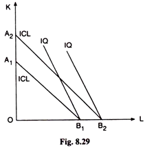
(3) and (5) give us that the numerical slope of the ICLs (=1/2) is smaller than that of the IQs (= 1), i.e., the IQs are steeper than the ICLs (Fig. 8.29). Therefore, here the firm’s output-maximising equilibrium subject to cost constraint would occur at the corner points of the ICLs, like B₁, B₂, etc., on the horizontal axis of Fig. 8.29. That is why here the horizontal axis (for L ≥ 0) would be the firm’s expansion path.

Example 3.

A firm use two inputs X and Y for producing its output. The production function of the firm is q = f (x, y) = xy, and the market prices of the two inputs are given to be Rs 20 and Rs 10, respectively. Find the input combination the firm should use to obtain the maximum possible output with the help of an expenditure of Rs 2,000, and also find what would be the maximum possible output.

Solution.

The production function of the firm is

q = f(x, y) = xy               ……….(1)

and the cost constraint is

C° = r_X x + r_Y y

or, 2,000 = 20x + 10y   ………..(2)

Here the relevant Lagrange function for obtaining the required input combination is

V = xy+ λ(2,000-20x-10y)   ………….(3)

where λ is the Lagrange multiplier.

Now, the first-order conditions for constrained output maximisation are

Putting this value of y in (6), we obtain

40 x = 2,000 => x = 50 units

and putting the value of x in (7), we obtain

y = 2 x 50= 100 units.

Therefore, the FOCs give us that the firm would have to use the input combination (x = 50 units, y = 100 units) in order to produce the maximum possible output, and putting the values of x and y in the production function (1), we obtain the maximum possible amount of output to be q = 50 x 100 = 5,000 (units) we may also verify the second-order condition given by

f_xx f²_y ^_ 2f_xy f_x f_y + f_yy f²_x < 0               …………..(8)

by putting the values f_x = y, f_y = x, f_xx = 0, f_yy = 0 and f_xy = f_yx = 1 in (8), we obtain: the left-hand side of (8) = – 2xy < 0 (v x = 50 > 0 and y =100 > 0). Therefore, the SOC is also verified.

Example 4.

If the production function of the firm is q = (x + 2) (y + 1) and the prices of the inputs are p_x = Rs 10 and p_Y = Rs 5, then find the least cost combination of producing 200 units of output and find the values of the amount of minimum cost.

Solution.

We are given the production function of the firm to be

q = (x + 2) (y + 1)            ………….(1)

Since the firm would have to produce a fixed 200 units of output, the output constraint would be:

q° = (x + 2) (y + 1)

or, 200 = (x + 2) (y + 1)            …………….(2)

Also, since p_X = Rs 10 and p_Y = Rs 5, the cost equation of the firm is

C = 10x + 5y                 …………..(3)

where C stands for any amount of money to be spent on the two goods.

Now, the relevant Lagrange function for constrained cost minimisation is

Z= 10x + 5y + μ[200-(x + 2)(y + 1)]              …………..(4)

Therefore, the first-order conditions (FOCs) for minimum cost are

Example 5.

A firm producing X from factors A and B can use either of the two production processes.

The production functions are:

Process I:

X = a A^.25 B^.75

Process II:

X = A^.75 B^.25

The price of A is Re 1. Let the price of B be P.

(i) At what price of B will the firm be indifferent between the two processes?

(ii) If the price of B is higher than that calculated in (i), which process will the firm use?

Solution:

(i) From the given information, we may write the cost equation of the firm as

If the firm is to be indifferent between the two processes, then for any given cost level C₀, outputs, i.e., the values of X in the two processes as given by (11) and (18), should be equal, i.e., we should have

i.e., we should have the price of input B as P = a².

(ii) (19) and (20) give us that, for P = a², we obtain equality (19). Now if P becomes greater than a², then factor P ⁷⁵ in the denominator of left-hand side (LHS) of (19) would increase by a greater proportion than the factor P²⁵ in the denominator of the right-hand side (RHS) of (19). Consequently, the LHS of (19) or output in process I would become smaller than the RHS of (19) or output in process II, and therefore, now process II would be preferred.

Example 6.

A firm may use two production processes Q_c = K^1/3_C L^2/3_C and Q_D = K^1/2_D L^1/2_D to produce an output. The total quantities of capital (K) and labour (L) that it may use are A and B, respectively. How the inputs should be distributed between the two processes so that the total output Q = Q_C + Q_D is maximised?

Solution.

The two production processes that the firm may use are

(11) gives us that, to maximise Q, K and L should be distributed between the two processes in such a way that the ratio of K_C to K_D, should be equal to 1/2 of the ratio of L_C to L_D (provided the second-order condition for constrained output maximisation is satisfied).

Let us suppose that

Eqns (14) and (15) give us the quantities of K and L that should be used in the two processes given m = K_C/K_D and 2m = L_C/L_D.

It may be noted here that we do not have any unique solution regarding the distribution of K and L between the two processes (given the arbitrariness of the value of m). But the solution at any value of m must satisfy (11).

Example 7.

A craftsman spends the first part of everyday sharpening his tools and the second part working with these tools. His total output is Y = X^1/4₁ X^3/4₂ where X₁ and X₂ denote the number of hours devoted to sharpening and use of tools, respectively, [X] + X₂ is fixed]. What is the efficient way for him to divide his time between these two activities.

Solution.

The production function is given to be

Y = X^1/4₁ X^3/4₂ = f(X₁, X₂),           …………..(1)

where X₁ = number of hours devoted to sharpening his tools = constant and

X₂ = number of hours devoted to using these tools = constant

and Y = quantity of output produced per period.

Let us suppose that the total number of hours available per day is T = constant.

Therefore, the craftsman would have to maximise Y in (1) subject to the constraint

T = X₁ + X₂                              …………..(2)

Now, the relevant Lagrange function here is

Condition (7) is the 1st order or necessary condition for constrained output maximisation. It shows us that the efficient way for the craftsman to divide his time between the two activities is to devote thrice as much of time to working with his tools as to sharpening them.

Let us now see whether the second-order or sufficient condition is satisfied at the point where the first-order condition is satisfied. The SOC is given by

Example 8.

If the marginal product of L is MP_L = 100 K – L and the marginal product of K is MP_K = 100 L – K, then find the maximum possible output when the total amount that can be spent on L and K is $ 1,000, and the price of L (P_L) is $2 and that of K (P_K) is $5 with comments, if any.

Solution.

Let us suppose, the production function is

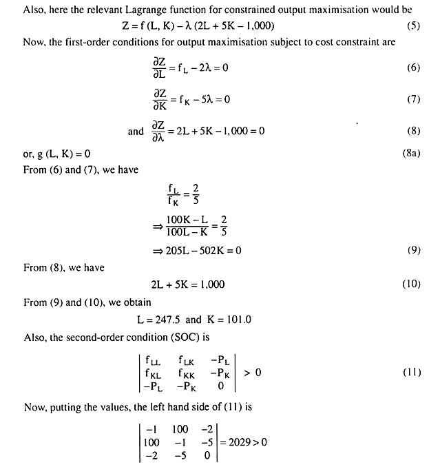
Therefore, the SOC is satisfied, and so, the output-maximising quantities of the inputs are

L = 247.5 (units) and K = 101.0 (units).

Now, the maximum output may be obtained here as total product of labour (TP_L) at L = 247.5, K remaining fixed at K = 101.0, or, it may be obtained as total product of capital (TP_K) at K = 101.0, L remaining fixed at L = 247.5.

In the first case, the MP_L (= f_L) function would have to be integrated over the interval 0 and 247.5 units of L, and, in the second case, the MP_K (= f_K) function would have to be integrated over the interval 0 and 101.0 units of K. Let us proceed along the first course and obtain the amount of maximum output in the following way.

Comments:

In order to obtain the maximum output we might as well integrate the MP_K function over the interval 0 and 101.

Although in both cases (of integration of the MP_L function and that of the MP« function), the (maximum) output quantity would be obtained at L = 247.5 and K = 101, the results would be different (may be by a relatively small extent) because in the first case labour is treated as a variable input and capital as a fixed input and in the second case capital is treated as a variable input and labour as a fixed input.

Example 9.

An entrepreneur uses one input to produce two outputs subject to the production relation x = A (q₁^α + q₁^β) where α, β > 1. He buys the input and sells the outputs at fixed prices. Express his profit-maximising outputs as functions of the prices. Prove that his production relation is strictly convex for q_b q₂ > 0.

Solution.

The production relation of the firm is given to be

Example 10.

(a) The production function is X = AK^α L^β, where α + β < 1. Show that there are decreasing returns to scale and prove that the total product is greater than K times the marginal product of K plus L times the marginal product of L, where K and L are the quantities of factors K (capital) and L (labour), respectively.

(b) Suppose a production function, X = f (K, L), shows constant returns to scale. Then, if the marginal productivity of labour (L) is greater than its average productivity, the marginal productivity of capital (K) is negative.

(c) Prove that the elasticity of factor substitution is unity for Cobb-Douglas technology. Is the assumption of constant returns necessary for your proof.

Solution.

(a) The production function is

X = AK^αL^β                           ……….(1)

where α + β < 1              ……….(2)

Here, if we increase both the input K and L, t times, where t is a positive real number, then the output is obtained to be

That is, here, if inputs are increased by a certain proportion, then output increases less than proportionately. So, here, we have decreasing returns to scale.

Again, K times MP_K plus L times MP_L is

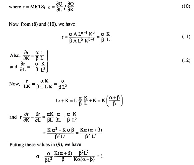
Since, while proving σ = 1 in the case of Cobb-Douglas technology, we have not needed the proviso α + β = 1, assumption of CRS is not necessary for this proof.

Example 11.

The following information is given for a firm which is producing a single output (X) by using two inputs, capital (K) and labour (L). One more unit of L could increase output by 200 units whereas one more unit of K could raise output by 150 units. Moreover, P_K = Rs 25.00 and P_L = Rs 10.00. Is the firm employing the optimal input bundle for its current output? If not, which would be the optimal direction of change?

Solution.

We are given here

MP_L = 200 (units), MP_K = 150 (units), P_L = 10 (Rs) and P_K = 25 (Rs).

Now, as we know, the first-order condition for optimum input bundle is

where MP_L/P_L = marginal product (MP) of money spent on labour

and MP_K/P_K = marginal product of money spent on capital.

But here at the particular input bundle with MP_L = 200 and MP_K = 150, we have

MP_L/P_L = 200/10 = 20 and

MP_K/P_K = 150/25 = 6

That is, here we have MP_L/P_L > MP_K/P_K, or, the MP of money spent on labour is greater than the MP of money spent on capital, and, therefore, here the condition (1) for optimum input bundle is not satisfied. Therefore, the firm is not employing the optimum input bundle.

Since MP of money spent on labour is greater than the MP of money spent on capital, the firm should go on spending more on labour and less on capital till the two MPs become equal. This is the optimal direction for change.