Production Possibility Curve under Constant and Increasing Costs

A production-possibility curve (Samuelson) in the international trader literature is also known as the substitution curve (Haberler), production indifference curve (Lerner) and transformation curve.

It is a simple device for depicting all possible combinations of two goods which a nation might produce with a given resources.

The slope of the curve at any point represents the ratio of the marginal opportunity costs of the two commodities. That is, the marginal opportunity cost of an extra unit of one commodity is the necessary reduction in the output of the other.

The shape of the curve depends on the assumptions made about the opportunity costs. It may be assumed that opportunity cost is constant. In this case the amount of G given up to allow additional production of D is the same regardless of the amount of G and D being produced. In contrast, it may be assumed that the opportunity cost is one of increasing cost; this means that every time an additional unit of D is produced, ever increasing amount of G must be given up in order to provide the resources for expanding D’s output.

Constant Costs:

The marginal rate of transformation (MKT) is the amount of one good G which must be given up in order to release resources necessary to produce an additional unit of second good D.

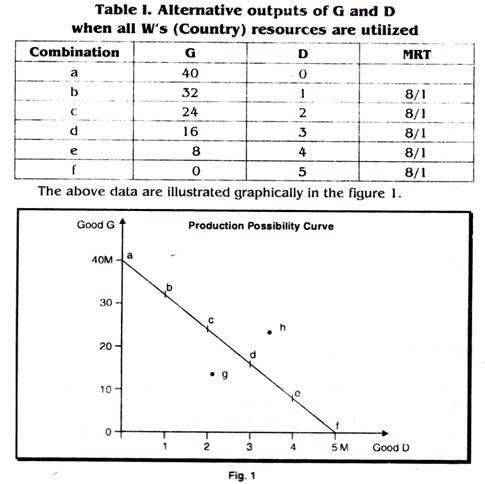
In the table, each additional unit of D has the same cost in terms of G, resources capable of producing 8 units of G must be diverted to increase output of D by one unit, regardless of the level of production of Gand D. Constant cost means that the MRT is constant. It is the result of each factor of production being equally effective in producing both goods, that is, a factor of production is not more suited to the production of one good than two other.

The production possibilities curve (MM) then shows all possible combinations of two commodities which country W might produce. The particular combination to be chosen lies on the curve. Points inside the curve such as (g) -represent outputs of less than full employment and are therefore not considered. Points beyond the curve, such as (h), require more resources than the country possesses and are therefore also beyond consideration.

The full employment output under consideration must be on the production possibilities curve. The slope of the production possibilities curve is the marginal rate of transformation. The slope shows the reduction required in one commodity in order to increase the output of the second commodity. Since the MRT is constant the slope must be constant and thus the production possibilities curve must be straight line. It can be seen that the MRT of G for D is 8 to 1; reducing the output of D by one unit will provide resources sufficient to expand output of G by 8 units.

Country, Z has a comparative advantage in the production of D; less G has to be given up for each additional unit of D. On the other hand, country W has the comparative advantage in the production of G₁ less D has to be given up to produce an additional unit G.

With constant returns to scale, trade can take place only when each nation has a different MRT. The gains from trade for a particular nation depend on how much the international exchange rates differ from that nation’s MRT. The greater the difference, the greater is the gains from trade. The gains from trade rest further upon the amount of trade taking place. Obviously a larger volume of trade allows larger gains from trade and a greater increase in the standard of living.

Under constant cost, the exchange ratio is determined solely by costs; the demand determines only the allocation of available factors between the two branches of production, and hence the relative quantities of G and D which are produced. In this case, demand has nothing to be with the price.

Increasing Costs:

It would seem unlikely that most nations would be confronted with constant costs over the substantial range of production. Constant costs imply that all resources are of equal quality and that they are all equally suited to the production of both commodities.

Increasing opportunity costs mean that for each additional unit of G produced, ever-increasing amounts of D must be given up. At first as production G is increased, resources suited to G but not to D are used to increase greatly the output of G and reduce the output of D by little. But eventually, the resources being transferred are not well-suited to G but highly suited to D and consequently G’s production increases by little and D’s fall by a great deal.

Increasing opportunity costs can best be explained by the use of a table.

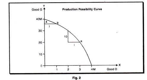
Suppose we take a given amount of land, labour and capital and experimentally find out how much G and D we can produce. If all our resources are devoted to the production of G, we find that we can produce 40 units of G . if we want 36 units of G, we find that we can have one unit of D, with all our resources fully employed. If we want two units of D, we can have only 30 units of G. With 3 units of D, we can have only 20 units of G. The first unit of D costs 4 units of G, the second 6 and the third 10.

The MRT of G for D is increasing, larger amounts of G must be given up for additional units of D. This is what is meant by increasing opportunity costs. When costs are increasing, the demand affects the exchange ratio also, since the relative costs the substitution ratio will vary with the relative demand for G and D. Given the combination of G and D which is demanded, the exchange ratio between them will equal their substitution ratio at that point. In other words, the ratio at which G and D will exchange against one another in the market will be equal to the ratio of their marginal costs. Any other situation would be one of disequilibrium: there will be an incentive to produce more G and less D or conversely. The data in the table may be represented graphically as a transformation curve.

First, a combination of 40 G and zero D is plotted in the figure 36 G and one of D etc.; the connected points yield a production possibilities curve, the slope of which is the mrt. The production possibilities curve is concave toward the origin, showing that the substitution rate is not constant but increasing.

At a combination of 20 G and 3 D, represented by point (a) in the figure, one unit of D may be substituted in production for 10 of G. But at the combination of 36 G and one D, represented by point (b) in the figure, the resources required to produce one D can be used alternatively to produce 4 additional unit of G. Now, the production possibilities curve shows all possible combination of G and D which can be produced at full employment. To be inside the curve is to be at less than full employment. There are not sufficient resources to go beyond the curve.

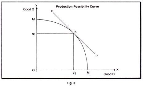
A price ratio must be introduced in our graph of production possibilities curve in order to determine the output of two commodities. With the assumption, that nation W has a closed economy the domestic price-ratio is drawn tangent to the production possibilities curve in the figure. The equilibrium point is at (K), where og¹ of G and od¹ of D are produced and consumed.

‘A straight line tangent to the transformation curve indicates the ratio of market prices of the two commodities, and the condition of tangency expresses equilibrium in production, that is, equality between prices and marginal costs stated in opportunity terms. Domestic demand conditions enter into this construction via community indifference curves, or simply as a consumption point determined by a given arrangement of production and income distribution.” In an open economy, the world price ratios enter to reveal the possible positions of equilibrium with international trade.

Finally, tangency of a line representing the equilibrium international price ratio to both transformation function and community indifference curve indicates equilibrium in exchange, that is:

(i) Equality domestically between the marginal rate of substitution in consumption and marginal rate of transformation in production, and

(ii) Equality of the value of exports and the value of imports.

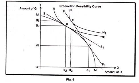
Suppose that if trade is opened with the outside world; G will be imported from abroad in exchange for D on the terms indicated by the slope of the FF line which is tangent at (V) to the production possibilities curve, MM and at (H) to another amount of consumption indifference curve of our country NN₁, which is higher than qq₁ and therefore taken to represent a greater total utility than qq₁. If the slope of FF₁ is taken to represent the equilibrium terms of exchange of G for D under foreign trade, our country will under equilibrium produce og₃ of G and od₃ of D; will consume og₃ of D and od₃ of D; and will import g₁ g₃ of G and export d₃ d₁ of D.

The amount of G and of D available to it for consumption will therefore both be greater under foreign trade then in the absence of such trade. Foreign trade will result in our country having available for consumption a combination of G and D which will be on a higher consumption indifference curve than q₁ q₁ and therefore will indicate a greater total utility than qq₁ though less may be consumed of one of the commodities under foreign trade than in the absence of such trade. Foreign trade therefore, necessarily results in gain. Such is the opportunity cost theory as applied to the problem of gains from trade.