Production in the Short Run with One Variable Input

In this article we will discuss about the Production in the Short Run with One Variable Input:- 1. Total, Average and Marginal Product of a Variable Input 2. Total Product of Labour (TP_L) Curve and the Law of Variable Proportions 3. The Average Product of Labour (AP_L) and the Marginal Product of Labour (MP_L) Curves—Derivation of the AP_L and MP_L Curves from the TP_L Curve and Other Details.

Contents:

1. Total, Average and Marginal Product of a Variable Input
2. Total Product of Labour (TP_L) Curve and the Law of Variable Proportions
3. The Average Product of Labour (AP_L) and the Marginal Product of Labour (MP_L) Curves—Derivation of the AP_L and MP_L Curves from the TP_L Curve and Other Details
4. Relation between the Average and Marginal Product of a Variable Input
5. Derivation of the MP_L – AP_L Relation—the Calculus Method
6. Returns to a Factor
7. Equilibrium of the Firm in Production with One Variable Input and Efficiency of the Second Stage of Production

1. Total, Average and Marginal Product of a Variable Input:

Total Product:

The firm uses a number of inputs to produce its output. If the firm varies the quantity of only one input, keeping the other input quantities unchanged, then the quantity of its output obtained at any quantity of the variable input is called the total product of the input.

For example, if the said variable input is labour and if it is obtained that the firm produces 42 units of output when it uses 6 units of labour along with the fixed inputs, then we say that the total product of labour is 42 units when 6 units of labour are used.

The schedule of total product obtained at different quantities of labour used by the firm is called the total product schedule of labour—it expresses the total product of the firm (i.e., the total quantity of output) as a function of the quantity of labour used. This function is called the total product function.

Columns (1) and (2) of Table 8.1 constitute the total product schedule or total product function of labour. This function may be written as

q = f (L)                           (8.8)

or, TP_L = f (L)                (8.9)

Here q or TP_L is the total product of the firm or the total product of labour and L is the quantity of labour used.

Average Product:

If we divide the total product of an input by the quantity used of it, we obtain the average product of the input. For example, if the total product of labour is 40 units per day when the firm uses 5 units of labour per day, then the average product of labour (AP_L) would be 40/5 or 8 units.

The average product schedule obtained at different quantities of labour used is called the average product schedule of labour—this schedule expresses AP_L as a function of labour. Columns (1) and (3) of Table 8.1 constitute the AP schedule of labour or the AP function of labour. We may express this function as

AP_L = q/L = f(L)/L = g(L)                    (8.10)

Marginal Product:

Marginal product of a variable input, say, labour (MP_L), is the increment in total product of labour (TP_L) obtained as a result of the use of the marginal (or an additional) unit of labour.

For example, if the TP_L be 32 units and 40 units, respectively, when the firm uses 4 and 5 units of labour, then the marginal product of labour (MP_L) at L = 5 units would be the increment in TP_L that would be obtained as a result of the use of the 5th unit of labour, and so here we would have MP_L = 40 – 32 = 8 units.

On the basis of the above definition of MP_L, we may write:

(MP_L)_{L = n units} = (TP_L)_{L = n units} – (TP_L)_L = _{n- 1 units} (8.11)

It is obtained from (8.11) that the firm’s MP_L would be positive or negative according as the firm’s total product rises or falls when an additional unit of labour is used.

Lastly, it follows from the above definition of MP_L that MP_L is the rate of change of total product of labour w.r.t. the quantity of labour used.

That is why we may write:

(8.12) gives us the marginal product of labour function and it also gives us that MP_L is the slope of the TP_L function or the TP_L curve.

Columns (1) and (4) constitute the MP_L schedule which gives us the marginal product of labour at different quantities of labour used. This schedule expresses the MP_L as a function of L.

2. Total Product of Labour (TP_L) Curve and the Law of Variable Proportions:

Total product of labour (TP_L) and the TP_L schedule. The total product of labour or the total product of the firm at any particular quantity of labour used can be known from the TP_L schedule and also from the TP_L curve, the latter being the graph of the former. A hypothetical TP_L curve of a firm has been given in Fig. 8.1. This curve gives us that TP_L at L = L₁ is L₁H and TP_L at L = L₂ is L₂S.

Now we have to remember certain points if we are to explain the shape of the TP_L curve. It has been found from the experience of production of goods and services that if the firm increases the quantity used of a variable input, say, labour, other input quantities remaining unchanged, then, initially, TP_L increases and at an increasing rate, i.e., initially, the slope of the TP_L curve while being positive, increases.

That is why, in the initial stage, the TP_L curve would be positively sloped and convex downwards. But if L increases beyond a certain quantity (beyond L = L₁ in Figure 8.1), TP_L increases but at a diminishing rate. That is why the TP_L curve now would be positively sloped and concave downwards.

Then at a certain L (at L=L₁), the TP_L becomes maximum and the TP_L curve reaches its highest point. Lastly, if L increases beyond this value, (i.e., L = L₂), TP_L would be diminishing and the TP_L curve would be sloping downwards towards right.

The Law of Variable Proportions (LVP):

The laws that the total product of the firm would follow when the firm increases the quantity of the only variable input (here labour), and when the proportion between the variable input and the fixed inputs varies. That is why these laws, taken together, are known as the law of variable proportions.

As it is obtained from above, the law of variable proportions (LVP) consists of three laws, those of increasing, diminishing and constant returns. Initially, production with one variable input (labour) follows the law of increasing returns.

According to this law, output would increase at an increasing rate as the quantity of labour increases. Graphically, this law is represented by the convex downwards segment of the TP_L curve (for example, the segment OH of the TP_L curve of Fig. 8.1, for 0 ≤ L ≤ L₁).

At the end of the stage of increasing returns, production follows the law of diminishing returns. According to this law, output would increase at a diminishing rate as labour is used more and more. Graphically, this law is represented by the positively sloped and concave downwards portion of the TP_L curve (for example, the segment HS of the TP_L curve for L₁ ≤ L ≤ L₂).

At the end of the stage of diminishing returns, i.e., at L = L₂, the firm’s output reaches the maximum. If the firm still increases its use of labour beyond L = L₂, the firm’s output diminishes and we have the negatively sloped portion of the TP_L curve. This is the stage of negative returns. If we assume that the firm does not have labour free of cost, this stage is not relevant for the firm’s decision-making.

Lastly, we may add that there may be a (small) stage of constant returns between the stages of increasing and diminishing returns. In this stage output increases at a constant rate as L increases, and the TP_L curve becomes an upward sloping straight line. Generally, this stage is found to be very small.

If this stage is not obtained, i.e., if diminishing returns set in as soon as the stage of increasing returns ends, we have a point of inflexion like the point H. At this point the TP_L curve changes its shape from being convex downwards to being concave downwards.

3. The Average Product of Labour (AP_L) and the Marginal Product of Labour (MP_L) Curves—Derivation of the AP_L and MP_L Curves from the TP_L Curve:

We have assumed that the firm uses only one variable input, labour, to produce its output. The AP_L and the MP_L curves are the graphs of the AP_L and the MP_L schedules (like those given in Table 8.1). The average and marginal products of labour at any L can be known from the AP_L and MP_L schedules and also from the AP_L and the MP_L curves.

The shapes of the AP_L and MP_L curves would be like the curves given in Fig. 8.2—their shapes would be like an inverted-U. The characteristic features of their shapes are obtained from the shape of the TP_L curve. Since, the shape of the TP_L curve reflects the law of variable proportions, the shapes of the AP_L and MP_L curves are also derived from this law.

We shall now explain how the AP_L curve is derived from the TP_L curve with the help of Fig. 8.2. In part (a) of this figure, at L = L₁ = OL₁, we have TP_L = L₁H and AP_L = TP_L/L = L₁H/OL₁ = the slope of the line OH which is called the guide line to the TP_L curve at point H.

Therefore, generally speaking, AP_L at any L would be equal to slope of the guide line to the TP_L curve at the corresponding point on it. For example, AP_L at L = L₂ and L₄ would be, respectively, the slopes of the guide line to the TP_L curve at the points R and E.

Now, it follows from the shape of the TP_L curve that as L rises, the slope of the guide line to this curve, i.e., AP_L, increases till it becomes maximum when the guide line touches the TP_L curve and thereafter as L rises, the slope of the guide line, i.e., AP_L, diminishes.

In Fig. 8.2(a), the guide line touches the TP_L curve at the point R or at L = L₂. We obtain, therefore, that AP_L rises as L rises till it becomes the highest at L = L₂ and then as L rises AP_L: diminishes. So in Fig. 8.2(b), we obtain the AP_L curve to be an inverted-U—it is a second degree curve and it reaches its maximum at L = L₂ or at the point G.

We shall now see how we may derive the MP_L curve from the TP_L curve. By definition, MP_L is the derivative of TP_L w.r.t. L, i.e., MP_L is the slope of the TP_L curve.

Therefore, initially, when the TP_L curve is convex downwards in the stage of increasing returns, we obtain that, as L rises, the slope of the TP_L curve rises, i.e., MP_L rises, and at L = L₁ or at the point of inflexion H on the TP_L curve, i.e., at the last point on its convex downwards portion, the slope of the TP_L curve, i.e., MP_L reaches its maximum.

Thereafter, as L rises and as we move along the concave downwards portion of the TP_L curve in Fig. 8.2(a), the slope of the TP_L curve or MP_L diminishes till it becomes zero at L = L₃ when the TP_L curve reaches its maximum, and thereafter as L rises MP_L becomes negative.

Therefore, in Fig. 8.2, we obtain the MP_L curve also, like the AP_L curve, to be an inverted-U second degree curve. Here the MP_L curve reaches its maximum at L = L₁ or at the point F, and the curve intersects the L-axis at L = L₃ when MP_L falls to zero, and thereafter the MP_L curve falls below the L-axis and MP_L becomes negative.

4. Relation between the Average and Marginal Product of a Variable Input:

We shall derive here the relation between the average and marginal product of a variable input, say, labour, with help of an easy example. Let us suppose that the firm uses 9 units of labour (L = 9) and produces 54 units of output [q = f (L) = 54], Therefore, here we have AP_{L = 9} = 54/9 = 6 units.

If the firm now uses one more unit of labour, keeping the other input quantities unchanged, i.e., if the firm now uses 10 units of labour, then the increment in total product would be the marginal product at L= 10, or MP_{L = 10}.

Now, if MP_{L= 10} > AP_L=9 , then AP_L would increase, i.e., we would have AP_L=10 > AP_{L = 9}. For example, if MP_L=10 = 7 (> 6), then we have AP_L=10 = 54 + 7/10 = 6.1 (> 6). That is, if MP_L > AP_L as L rises, then AP_L would increase.

Therefore, conversely, if AP_L rises as L rises, then we have MP_L > AP_L. This is the first point of the relation between MP_L and AP_L.

Again, if MP_{L= 10} = AP_{L = 9} (= 6), then we would have AP_{L= 10} = AP_{L = 9}, i.e., AP_L would remain unchanged. For, now, we have AP_L=10 = 54 +6/10 = 6 Therefore, we have obtained here that if as L rises, MP_L = AP_L, then AP_L would remain unchanged. Conversely, we get, if AP_L remains unchanged as L rises, then MP_L = AP_L. This is the second point of the relation between MP_L and AP_L.

Lastly, if MP_{L= 10} < AP_L=9 , if MP_{L= 10} = 5, say, then we would have AP_L=10 < AP_L=9. For now we would have AP_L=10 =54 + 5/10 = 5.9 (< 6). Therefore, here we have obtained that if, as L rises, MP_L < AP_L, then AP_L would diminish. Conversely, we have: if AP_L diminishes as L rises, then we should have MP_L < AP_L. This is the third point of the MP_L -AP_L relation.

The MP_L-AP_L relation that we have been able to derive above has been represented in Fig. 8.2(b). Here the shape of the continuous AP_L curve has been like an inverted-U and G is the maximum point of this curve. Therefore, at the point G (i.e., at L = L₂), AP_L would remain the same if L changes by an infinitesimally small quantity (since here the analysis is a continuous analysis).

This gives us MP_L = AP_L at the maximum point G on the AP_L curve, where L = L₂. This is the second point of the relation. Therefore, the point G or the maximum point on AP_L is the point of intersection between the MP_L and the AP_L curves.

Also, since the AP_L curve is an inverted-U and G (L = L₂) is its maximum point, we obtain that, to the left of G (for L < L₂), as L rises, AP_L also rises. Therefore, the first point of MP_L-AP_L relation gives us MP_L > AP_L or the MP_L curve lies above the AP_L curve when L < L₂.

Similarly, to the right of the point G (for L > L₂), as L rises AP_L declines. Therefore, the third point of MP_L– AP_L relation gives us MP_L< AP_L or the MP_L curve lies below the AP_L curve when L > L₂. Therefore, we have corresponding to the three points of MP_L– AP_L relation, we have three points of relation between the MP_L and AP_L curves.

These points are:

(i) The two curves intersect at the maximum point on the AP_L curve,

(ii) To the left of this maximum point, when the AP_L curve is upward sloping, the MP_L curve lies above the AP_L curve, and

(iii) To the right of this maximum point, when the AP_L curve is downward sloping, the MP_L curve lies below the AP_L curve.

5. Derivation of the MP_L – AP_L Relation—the Calculus Method:

We may derive the relation between the MP_L and the AP_L with the help of calculus also. Let us suppose that the production function of the firm which uses only one variable input, labour, is

q = f(L)                                             (8.13)

where L is the quantity of labour used per period and q is the quantity of output produced per period. By definition, the average and marginal product of labour (AP_L and MP_L) are

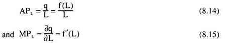
As we know, both the AP_L and the MP_L curves would be inverted-Us because of the law of variable proportions (LVP). We have shown these curves in Figure 8.2(b).

Since the AP_L curve is an inverted-U, it would reach its maximum at some L, and to the left and right of this maximum, the curve would be upward sloping (i.e., positively sloped) and downward sloping (i.e., negatively sloped), respectively. In Fig. 8.2(b), the AP_L curve has reached its maximum at the point G (when L = L₂). Therefore, we obtain

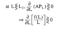
From (8.16), we obtain the following points of relation between the MP_L and AP_L and between the MP_L and AP_L curves as shown in Fig. 8.2:

(i) When L < L₂, we would have MP_L > AP_L. That is, to the left of the maximum point G on the AP_L curve, we obtain MP_L > AP_L, and the MP_L curve would be above the AP_L curve.

(ii) When L = L₂, we would have MP_L = AP_L. That is, at the maximum point G on the AP_L curve, we obtain MP_L = AP_L, and the MP_L and AP_L curves would intersect each other at this point.

(iii) When L > L₂, we would have MP_L < AP_L. That is, to the right of the maximum point G on the AP_L curve, we obtain MP_L < AP_L, and the MP_L curve would lie below the AP_L curve.

(iv) It follows from (i), (ii) and (iii) above that the MP_L curve is above the AP_L curve to the left of the point G and it is below the AP_L curve to the right of this point.

This gives us that the MP_L curve is downward sloping at the point G (L = L₂) which is the maximum point of the AP_L curve, and the MP_L curve, an inverted-U, must have reached its maximum at some point to the north-west or upwards towards left of point G where L < L₂.

This point, as we see in Fig. 8.2(b), is the point F (L = L₁ < L₂). If we compare the points F and G, we find that L at point F = L₁ < L at point G = L₂ and MP_L at point F = maximum MP_L = L₁F > AP_L at point G = maximum AP_L = L₂G. From this we obtain that the MP_L curve reaches its maximum earlier (at a lower L) than the AP_L curve and the maximum MP_L is greater than the maximum AP_L.

6. Returns to a Factor:

The Three Stages of Production and the Law of Variable Proportions (LVP):

In the theory of production with only one variable input, the economists have distinguished between three stages of production, depending on the nature of the response of output to changes in the quantity of the variable factor (labour). The first stage of production is the stage of MP_L being greater than AP_L.

Since AP_L rises so long as MP_L remains greater than AP_L, this stage is also the stage of rising AP_L and the stage ends at the maximum point [G in Fig. 8.2(b)] on the AP_L curve. In Fig. 8.2, the range of this stage is 0 ≤ L ≤ L₂, i.e., so long as labour employment is between 0 and L₂, the production is in the first stage. This stage is also called the stage of increasing returns.

The second stage of production is the stage of MP_L being less than AP_L, while remaining non-negative. The second stage begins where the first stage ends, i.e., the stage lies to the right of the maximum point G (Fig. 8.2) on the AP_L curve and runs up-to the point of intersection L₃ between the MP_L curve and the L-axis.

The range of the stage is L₂ ≤ L ≤ L₃. Since this stage lies to the right of the maximum point G on the AP_L curve, both AP_L and MP_L fall in this stage as L rises. This stage is also known as the stage of diminishing returns.

Finally, the third stage is the stage of negative MP_L. This stage begins where the second stage ends, i.e., the stage lies to the right of the point L₃ in Fig. 8.2. The range of L for this stage is L > L₃. This stage may be called the stage of negative returns.

Conditions for the Applicability of the Law of Variable Proportions:

There are two main conditions for the applicability of the LVP:

(i) The production function or the technology of the firm should remain unchanged. For, if there occurs continuous improvement in technology, returns would be obtained at an increasing rate even if the use of the variable factor (labour) goes on increasing indefinitely.

(ii) The question of applicability of LVP arises only when the inputs can be used in variable proportions. There may be some areas of production where the inputs are to be used in a fixed ratio. In these areas if the use of the variable factor is increased and that of all other factors remains constant, the resulting change in output would be zero.

Therefore, here, the marginal product of the variable factor would be zero—it would not be diminishing, nor increasing.

Explanation of the Law of Variable Proportions:

The LVP states that if the use of a factor of production (labour) increases, that of all other factors of production remaining constant, then returns would be obtained first at an increasing rate, then at a diminishing rate and then at a negative rate. Explanation of LVP requires the explanation of all the three phenomena of increasing, decreasing and negative returns.

Increasing Returns:

The first stage of production is the stage of increasing AP_L and this stage is known as the stage of increasing returns. In this stage, the range of labour use is 0 ≤ L ≤ L₂ in Fig. 8.2. The portion of the TP_L curve from the point of origin to point R represents this stage of production. The total rising portion of the AP_L curve falls in this stage.

Now, why do we get increasing AP_L in this stage? This is because, in the initial stages of production, the firm uses much less of labour in relation to its fixed inputs. Therefore, as the use of labour increases in this stage the fixed inputs are used more and more intensively and effectively.

That is why in this stage, the increase in the use of labour results in an increase in production by a larger proportion which gives us an increase in AP_L.

We have to note here that in the initial stages the firm uses a relatively small quantity of labour, but the fixed input quantities with the firm are much larger than what are needed initially. This is because of two reasons.

First, in general, the quantity of output produced initially happens to be relatively small.

Second, the fixed inputs like the factory building and machines and appliances are indivisible for technological reasons and their size cannot be reduced below a certain minimum. That is, no matter however small the quantity of output is initially, and however small the quantity of labour used, fixed inputs used cannot be reduced accordingly.

Apart from the indivisibility of the fixed inputs, another cause of increasing returns is the specialisation and division of labour that can be put into practice as the use of labour increases in the initial stages to produce increasing quantities of output.

Decreasing Returns:

The stage of production—the second stage as we know—when both AP_L and MP_L are decreasing as the use of labour increases is known as the stage of diminishing returns. In this stage the quantity of labour used (L) lies in the range L₂ ≤ L ≤ L₃ in Fig. 8.2. The corresponding segment of the TP_L curve runs from the point R to the maximum point of the curve, viz., point S.

We have to explain why the second stage is the stage of diminishing returns. In the first stage, as the use of labour increases, the fixed inputs are used more and more intensively and effectively.

But if the quantity of labour used becomes more than a certain quantity, which is L₂ in Fig. 8.2, there develops a shortage of fixed inputs in relation to labour. That is why if the use of labour is increased now, output would increase in a smaller proportion. Consequently, both AP_L and MP_L would fall as L increases.

It is clear from the above analysis that increasing returns in the first stage result from the indivisibilities of fixed inputs. Similarly, decreasing returns in the second stage are also caused by the same indivisibilities.

In the first stage, fixed inputs are plenty in relation to labour owing to indivisibilities, leading to increasing AP_L, and in the second stage, when a shortage in fixed inputs develops, their quantities cannot be increased (in the short run) also owing to indivisibilities of these inputs, resulting in decreasing AP_L and MP_L.

Prof. Joan Robinson (1903—83) has gone deeper into the causes of diminishing returns. She tells us that diminishing returns are obtained because the factors of production are not perfect substitutes of each other.

If the variable factor, labour, had been a perfect substitute for the fixed inputs, then it might have been possible to make up for the deficit of the fixed inputs by using more of labour and in that case we might have obtained constant returns in place of diminishing returns. Therefore, according to Prof. Robinson, diminishing returns are caused by limited substitutability between the factors of production.

Negative Returns:

In the third stage of production the MP_L is negative. This stage is known as the stage of negative returns. In this stage the TP_L diminishes as L increases. Here the range of labour use is L > L₃ in Fig. 8.2.

The segment of the TP_L curve corresponding to this range is one that lies to the right of its maximum point. We may explain the negative returns to labour in this way. In the second stage, there is shortage of fixed inputs.

This causes both the MP_L and AP_L to be diminishing. But if the use of labour increases beyond a certain point, shortage of fixed inputs in relation to labour becomes so large or the employment of labour in relation to the fixed inputs becomes so large that now the TP_L starts falling or MP_L becomes negative. Exactly this happens in the third stage where L be­comes greater than L₃.

7. Micro-Economics, Production Theory, Short Run Production, One Variable InputEquilibrium of the Firm in Production with One Variable Input and Efficiency of the Second Stage of Production:

Here we shall assume that the firm uses only one variable input (labour) along with some fixed inputs to produce its output. We shall now discuss how the firm determines how much of labour to buy and what quantity of output to produce.

The assumptions:

We shall assume:

(i) The firm is using only one variable input, labour, along with other fixed inputs. The short-run production function of the firm is

Q = f (L)                                     (8.17)

(ii) The price P of the product is given and constant, and the firm can sell any quantity of output at this price. That is, there is perfect competition in the product market.

(iii) The price of labour, i.e., the rate of wage (W), is also given and constant, and the firm can buy any quantity of labour it requires, at this wage in the perfectly competitive labour market.

(iv) The firm’s goal is to buy labour and produce the product in appropriate quantities so that its profit is maximised.

Definitions:

Before we proceed to establish the decision-making rule of the firm, let us define certain concepts and ideas that we have to use here.

First, we should note that profit (π) of the firm per period is the difference between its revenue and cost per period. Revenue is obtained from the sale of the firm’s output which again is produced by the variable input, labour (along with some fixed inputs).

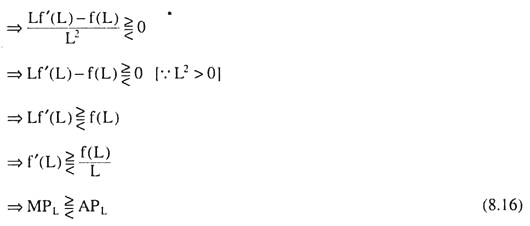
So revenue here is a function of labour quantity used (L) and is known as total revenue product of labour (TRP_L). Fixed input quantities being fixed, would not enter into this function. Corresponding to TRP_L, we would have

And MRP_L (marginal revenue product of L) = MP_L x P (^._.^. P is constant) = VMP_L

Here VMP_L is the value of MP_L. Both ARP_L and MRP_L are function of L.

On the cost side, total cost (TC) is made up of total expense for labour (TE_L) and total fixed cost (TFC) for the fixed inputs. TE_L is a function of labour quantity purchased (L).

Corresponding to TE_L, we would have

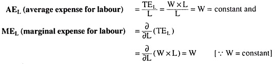
Both AE_L and ME_L are functions of L.

The Profit Function of the Firm and Profit-maximisation:

Here, the profit function of the firm would be

So π would have to be maximized w.r.t. L. Since TFC is constant w.r.t. L, or, Q (the firm would have to bear TFC even if L, or, Q is zero), we can maximize π

If we maximize TRP_L (L) = π_L, say.

The first-order condition for maximum π_L (and of maximum π) is

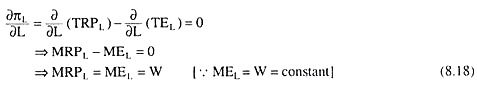
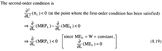
Conditions (8.18) gives us that, at any given W, π_L would be maximised at that L at which the firm would remain on the MRP_L curve. For example, at W = W₀, the firm’s π_L would be maximised at L = L₀. In other words, profit- maximisation requires that the firm’s demand curve for labour will be its MRP_L curve. However, condition (8.19) requires that at this L, the MRP_L curve should be sloping downward towards right.

Therefore, taken together, these two conditions require that at any W, π_L would be maximised at some point on the downward-sloping segment of its MRP_L curve. For example, in Fig. 8.3, at W = W₀, the firm would be in profit-maximising equilibrium at the point E₀ employing L₀ units of labour. Output at this L would be Q₀ = f (L₀) units [by virtue of (8.17)].

π_L Should be Greater than Zero:

But one important point we should remember here. If at the π_L-maximising point, maximum n:_L is negative i.e., if TE_L > TRP_L, the magnitude of TE_L-TRP_L being minimum, then the firm would not be able to recover even its variable cost (or, labour expenses) with its revenue or TRP_L. Under the circumstances, it would shut down its operations.

This is because, in the short run, the firm cannot avoid bearing the fixed cost, but it can avoid the cost for the variable input, labour, by reducing its output to zero. We may also note that, in the event of facing losses, the task of profit maximisation becomes one of loss minimisation. By shutting down its operations, the firm would be minimising its loss which would now be equal to the amount of its fixed cost.

The firm’s optimum point:

Therefore, the optimum point of the firm becomes the point of π_L-maximisation subject to the condition:

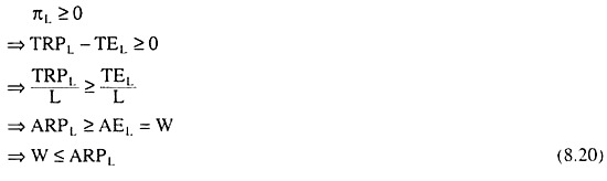
This last condition gives us that, at any W ≤ ARP_L, i.e., at any W ≤ W* in Fig. 8.3 (where W* = maximum ARP_L), or, at the corresponding L ≥ L₂, the firm would be in equilibrium at the appropriate point on the downward-sloping segment of its MRP_L curve, and at any W > ARP_L, i.e., at L < L₂, it would shut down.

The MRP_L cannot be Negative:

Also, in the real world, W ≠0 and at W ≥ 0 and MRP_L < 0, the firm would run into a loss on the marginal unit(s). So the firm cannot be in equilibrium at any point where MRP_L is negative, i.e., it cannot be in equilibrium at any L > L₃.

The Final Optimisation:

In production with one variable, the firm may be in profit-maximising (or loss-minimising) equilibrium at some point on the stretch of its MRP_L curve that starts on and from the maximum point (G) on the ARP_L curve and ends at the point of intersection (L₃) between the MRP_L curve and the L-axis. The corresponding range of labour employment is L₂ ≤ L ≤ L₃ in Fig. 8.3.

Efficiency of the Second Stage of Production:

In Fig. 8.3, ARP_L is maximum at L = L₂. This implies AP_L is maximum at L = L₂, since ARP_L = AP_L x P where P is constant. Also, MRP_L is equal to zero at L = L₃ implies MP_L is zero at L = L₃, since MRP_L = VMP_L = MP_L x P where P is a non-zero constant.

In other words, the stretch of the MRP_L curve from the maximum point on the ARP_L curve to the point where the MRP_L curve meets the L-axis corresponds to the stretch of the MP_L curve, in Fig. 8.2(b), from the maximum point of the AP_L curve at L = L₂ to the point where the curve meets the L-axis at L = L₃.

This latter stretch of the MP_L curve is, by definition, the second stage of production. Therefore, that production can occur only at L₂ ≤ L ≤ L₃, i.e., only in the second stage. That is why the second stage of production is the economically efficient stage of production.

It is important to note here, that the rising portion of the SMC curve of a firm corresponds to the falling portion of the MP curve of the variable input(s), and so, it follows from above that a particular segment of the rising portion of the SMC curve would correspond to the economically efficient second stage of production (which is again a particular segment of the falling portion of the MP curve).

In other words, the point at which a profit-maximising firm would operate in equilibrium must lie on the upward- sloping portion of its SMC curve.