
Some of the the important condition for Cost Minimising and Output Maximising Input Combinations are listed below:
Condition # 1. First-Order or Necessary Condition:
Both the points at which the firm’s cost-minimising input combination subject to an output constraint and output-maximising input combination subject to a cost constraint are obtained, are the points of tangency between an isoquant (IQ) and an iso-cost line (ICL) like the points T2, S3 and R4 in Fig. 8.12.

At such a point of tangency, we obtain the slope of the IQ (negative) = the slope of the ICL (negative) => the numerical slope of the IQ = the numerical slope of the ICL.
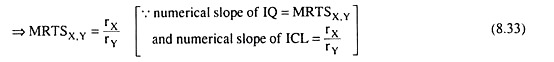
Equation (8.33) is the first-order or necessary condition, not the sufficient condition, for constrained cost minimisation or constrained output maximisation (i.e., for optimisation). Let us discuss the economic significance of this condition with the help of Fig. 8.12.
Since the ratio of the prices of the inputs is the marginal rate of substitution (MRS) of input X for input Y obtained on the basis of their relative market prices, the condition (8.33) for optimisation may be written as
MRTSX,Y = MRSX,Y in the market (8.34)
Economic interpretation for this may be given as follows.
ADVERTISEMENTS:
Let us suppose first that the firm’s cost constraint is given by the ICL, L3M3, and the firm intends to maximise output subject to the cost constraint. Let us also suppose that initially the firm is at the point V2 on L3M3 lying to the northwest of the point of tangency S3. At V2, the numerical slope of the isoquant IQ2 (= 5 say) is greater than the numerical slope of the iso-cost line L3M3 (= 2, say).
Here, if the firm leaves the point V2 and moves down southeastward along the line L3M3, to the point A and uses an additional unit of X, then it can use 2 units less of Y and still keep its cost unchanged. On the other hand, if it leaves the point V2 and moves southeastward along the curve IQ2 and uses 5 units less of Y and 1 unit more of X, then its quantity produced would remain the same as at the point V2.
Therefore, at the point A where the firm uses 1 unit more of X and only 2 units less of Y, its output would be more than that at the point V2. That is, the point A would lie on an IQ (shown by the broken line) which is higher than IQ2. Therefore, the firm would leave the point V2 on the ICL, L3M3, and move down southeastward to the point A (on a higher IQ, but, at the same cost).
Again, if at the point A also, the numerical slope of the IQ happens to be more than that of L3M3, then in order to produce more at the same amount of cost, the firm would again move southeastward along the line L3M3, leaving the point A. The process of the firm moving southeastward along L3M3 would continue till the firm arrives at the point S3 where the ICL, L3M3, would touch an IQ (here IQ3).
ADVERTISEMENTS:
Similarly, we may establish that if the firm initially happens to be at some point on L3M3 that lies to the southeast of the point of tangency, S3, then with a view to produce more at the given cost, the firm would go on substituting the input Y for X and moving northwestward along the line L3M3 till it reaches the point S3. Thus, the firm would be able to produce the maximum possible output at the given cost level of the ICL, L3M3, only when it is at the point of tangency, S3.
Next, let us suppose that the firm’s output constraint is given by IQ3 and the firm intends to minimise cost subject to the output constraint. Let us also suppose that, initially the firm is at any point S2 on IQ3 that lies to the northwest of the point of tangency S3. At S2, we obtain: the numerical slope of the IQ (= 6, say) > the numerical slope of the ICL (= 2, say).
Here if the firm moves southeastward along the IQ from S2 to B, and uses 1 additional unit of input X, then its output would remain unchanged even if it uses 6 units less of Y. Since, in the market, the value of 1 unit of X = the value of 2 units of Y, the firm’s cost of producing the same output (at B) would diminish by the market value of 4 units of Y. That is, at the point B, the firm would come down on a lower ICL (given by the broken line).
Now, if the numerical slope of IQ3 is again more than that of the ICL at the point B, then with a view to reducing the cost of production, the firm would move further southeastward along IQ3, and the process would continue till the firm moves down to the point of tangency, S3, between IQ3 and ICL3.
Similarly, it may be shown that if the firm is, initially, at a point on IQ3 that lies to the southeast of S3, then in order to reduce the cost of production of the given output of IQ3, it would go on substituting the input Y for X and it would go on moving northwestward along IQ3 till it reaches the point S3. Therefore, the cost of production of the output q3 along IQ3 would be the least at the point of tangency S3.
We have seen in the above analysis that if the firm is initially not at the point of tangency between an IQ and an ICL, then for the sake of optimisation, i.e., for maximising output subject to a given cost, or, for minimising cost subject to a given output, it would have to move to the point of tangency along an ICL or an IQ.
Once the firm reaches the point of tangency, it would not be possible for it, by moving away from this point, to increase its output further, given the cost constraint, or to reduce its cost further, given the output level. This is because, at the point of tangency, the ICL and the IQ are of equal slope.
Some other forms of the first-order condition and their economic interpretation
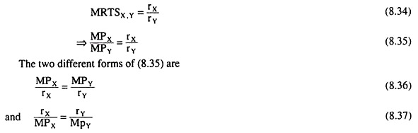
We may express the condition (8.33) for the firm achieving minimum cost or maximum output in some other forms also:
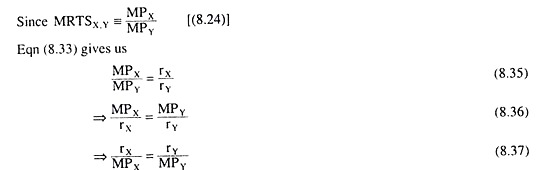
We have, therefore, obtained the four different forms of the first-order or necessary condition for constrained minimisation of cost or constrained maximisation of output. Since MRTSX,Y = MPX/MPY, equation (8.35) has the same economic interpretation as (8.34). We may now proceed to interpret the forms (8.36) and (8.37) of the optimisation condition.
Since MPX/rX and MPY/rY the marginal products (MPS) of money spent on inputs X and Y, respectively (see the box below), equation (8.36) gives us that if the firm is to have maximum output subject to a cost constraint, then the MP of money spent on each input should be the same, and the firm should distribute its money on purchasing the inputs accordingly.
 For if the firm acts otherwise so that, say, MPX/rX becomes greater MPY/rY than then the firm would spend more money on the input X and buy more of X and it would spend less money on Y and buy less of Y, for the MP of money is greater in the former channel.
Now, as the firm spends more money on X and uses more of X, and spends less money on Y and uses less of Y, MPX would fall and MPY would rise because of the law of diminishing marginal product, and so MPX/rX would fall and MPY/rY would rise (rX and rY being constants), The process would go on till the firm has shifted enough money from Y to X so that MPX/rX has become equal to MPX/rX.
ADVERTISEMENTS:
Once this equality is obtained, any further shifting of expenditure from Y to X, or otherwise, would not result in an increase in output, and so, output has attained the maximum possible level.
Similarly, if, initially, MPX/rX is less than MPY/rY, the firm would spend less on X and more of Y till MPX/rX rises and MPY/rY falls sufficiently to become equal to each other. Therefore, how the condition (8.36) may be interpreted.
Let us now come to condition (8.37). Here rX/MPX gives us the marginal cost (MC) of the output of the firm when it uses an additional unit of input X. Similarly, rY/MPY is the MC when the firm uses an additional unit of input Y. (See the box below).
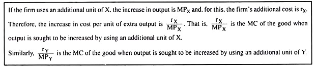 Therefore, condition (8.37) gives us that if the firm is to minimise the cost of production of a given amount of output, it would have to use that combination of the inputs X and Y for which we would obtain rX/MPX = rY/MPY.
ADVERTISEMENTS:
For if rX/MPX < rY/MPY, then the firm’s marginal cost of producing the good would decrease if the firm uses more of X and less of Y. Therefore, with a view to minimising the cost of production of a given amount of the good, the firm would use Y in a smaller quantity and X in a larger quantity and move southeastward along the IQ for the given output.
Consequently, the MPX would fall and rX/MPX would rise and MPY would rise and rY/MPY would fall, because of the law of diminishing marginal product. The process would go on till the rX/MPX and rY/MPY become equal to each other, and the IQ touches an ICL.
Once the firm reaches this tangency point it would no longer be possible to decrease the cost by using more of X and less of Y, i.e., now the cost of producing a given output would be minimum.
Similarly, if the firm is initially at a point where we have rX/MPX > rY/MPY, on substituting the input Y for the input X till rX/MPX diminishes and rY/MPY increases sufficiently so that the two may become equal to each other. Therefore, (8.37) is the condition for making the cost of producing a given amount of output the minimum.
Condition # 2. The Second-Order or Sufficient Condition:
In the above discussion, we have seen that the conditions for producing the maximum possible output at a given cost and that for producing a given amount of output at the minimum possible cost are identical, and this condition is
ADVERTISEMENTS:
ADVERTISEMENTS:
We now know that (8.34) – (8.37) are different forms of the same condition and this condition is satisfied at the point of tangency of an IQ and an ICL. We have also seen that although (8.36) and (8.37) are identical, we can directly explain the former as the condition for constrained output maximisation and the latter as that for constrained cost minimisation.
Now, (8.34) – (8.37) are the different forms of the first-order or the necessary condition for constrained output maximisation and cost minimisation, but they are not the sufficient conditions.
In other words, although it is necessary for the firm to operate at the point of tangency between an IQ and an ICL for the sake of output maximisation or cost minimisation, operation at this point does not guarantee the fulfillment of its objective.
Actually, the point of tangency would guarantee the fulfillment of its objective only if the IQs are convex to the origin. That is, convexity of the IQs provides us with the sufficient condition for constrained output maximisation or cost minimisation. We may now establish this with the help of Fig. 8.13.
If we replace the assumption of diminishing MRTS (Sec. 8.7.3) by the assumption increasing MRTS, i.e., if we assume that as the firm uses more of X and less of Y, MRTSX Y increases monotonically, then the numerical slope of the IQs would increase as the firm moves downward towards right along an IQ, which in its turn would imply that the IQs would be concave to the origin. We have given such concave IQs in Fig. 8.13.

If the IQs are concave to the origin, then at the point of tangency, the firm would have minimum output, not maximum, subject to a cost constraint or maximum cost, not minimum, subject to an output constraint.
This is because at the point of tangency tike S2, the ICL of the firm, viz., ICL2, which is the cost constraint, takes it to the lowest possible IQ, viz., IQ2. On the other hand, if the output constraint is given by IQ2, then at the point of tangency S2, the firm would be on the highest possible ICL, viz., ICL2.
Therefore, that the point of tangency or equations (8.34) – (8.37) provide us with the necessary condition for optimisation but they are not sufficient. If optimisation is to be guaranteed, then the IQs would have to be convex to the origin, not concave.