Firms That Produces Multiple Products

In this article we will discuss about the Firms That Produces Multiple Products:- 1. Multi-Plant Firms 2. Firms with Multiple Products 3. Opportunities for Multiple Products 4. Policy (Criteria)on Multiple Products 5. Multiple Products Related in Consumption 6. Multiple Products that are Complements in Production 7. Multiple Products that are Substitutes in Production and Others.

Contents:

1. Multi-Plant Firms
2. Firms with Multiple Products
3. Opportunities for Multiple Products
4. Policy (Criteria) on Multiple Products
5. Multiple Products Related in Consumption
6. Multiple Products that are Complements in Production
7. Multiple Products that are Substitutes in Production 
8. Cost of Multiple Products
9. Allocate Cost Among Multiple Products

---

1. Multi-Plant Firms:

A monopolist can produce output in various plants having different cost conditions. The prob­lem faced by the firm is, therefore, how to allocate the firm’s desired level of production among these plants.

For the sake of simplicity, we may assume that the firm is having only two plants, A and B. Sup­pose at the desired level of output, the following situation prevails

MC_A < MC_B.

The firm should surely transfer output from the higher cost plant B to the lower cost Plant A. If the last unit produced in Plant B costs Rs. 9, but one more unit produced in Plant A adds only Rs. 6 to A’s cost, then that unit should be transferred from B to A. The transfer results in a cost saving of Rs. 3. In fact, the firm will continue to transfer output from B to A until

MC_A = M C_B.

The marginal cost of the two plants are equalized because of the operation of the law increasing marginal cost. As output is transferred out of B into A, the marginal cost in A rises and the marginal cost in B falls. Exactly the opposite happens when the following inequality holds:

MC_A> MC_B.

Output is transferred from A to B (i.e., less is produced in A and more in B) until

MC_A = MC_B.

It is easy to determine the total output of the firm. The firm’s total marginal cost curve is ar­rived at by summing up horizontally the marginal cost curves of both the plants. The total marginal cost curve is equated to marginal revenue curve in order to determine the profit maximizing output and price. This output is divided among the plants so as to equate the marginal cost for both the plants.

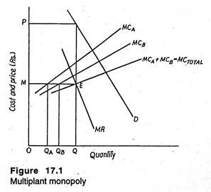
The situation is illustrated in Figure 17.1. The demand (AR) curve for the product is D, and margi­nal revenue is MR. The marginal cost curves for plants A and B are respectively MC_A and MC_B. The total marginal cost curve MC_TOTAL is the summation of the two.

Profit is maximized when this curve intersects the marginal revenue curve (at point E), giving an output of Q and a price of P. Mar­ginal cost at this output is M. For equalization of marginal costs, Plant A has to produce Q_A units and Plant B, Q_B units. Consequently, this allocation is the least-cost method of producing the desired lev­el of output.

Thus, we have extended the marginalize princi­ple of profit maximization in the case of allocation decision: profit is maximum if the firm produces the level of output and allocates production be­tween the plants so that

MR = MC Total = MC_A = MC_B.

The same principle can easily be generalized for more plants. But, in order to see how this principle could be implemented by a firm we may consider a simple two-plant example.

Example 1:

Suppose, a firm with some degree of market power produces its product in two plants.

It has ar­rived at the following linear estimates of the in­cremental (marginal) cost functions for the two plants:

MC_A = 28 + 4Q MC_B = 16 + 2Q

where the marginal costs were measured in rupees per unit and output was measured in thousand units. Here the estimated marginal cost function for Plant A (a plant built in 1968) is higher for every output than that of Plant B (a plant built in 1987); so Plant B is economically more efficient.

Summing horizon­tally (and, after a little manipulation), we obtain the following total marginal cost function:

MC Total = 20 + 4/3 Q

for outputs above 6,000 units.

Suppose that the estimated demand curve for the firm’s output is

Q = 114 – 3 P

The corresponding marginal revenue function is

MR = 38- 2/3 Q

By equating MR with total marginal cost, we get:

38- 2/3 Q = 20 + 4/3 Q

the profit-maximizing output for the firm is Q = 9 (i.e., 9,000 units). At this output, MR = MC, i.e., Rs. 32. For profit-maximization, the production of the 9,000 units should be allocated between Plants A and B so that the marginal cost of the last unit pro­duced in either plant is Rs. 32.

MC_A= 28 + 4Q = 32

MC_B = 16 + 2Q = 32

Thus, for Plant A, Q = 1. Thus, 1,000 units will be produced in Plant A. So, it logically follows that for plant B, Q = 8; so, 8,000 units (9,000 – 1,000) will be produced in Plant B.

Now, suppose that predicted demand falls. We may suppose that a new forecast of the demand for the firm’s output is Q = 96 – 3P

Given that the supporting marginal revenue func­tion is

MR = 32 – 2/3 Q

the firm’s profit-maximizing output falls to 6,000 units. At this level of output, MR and MC are equal, i.e., both are Rs. 28. Equating MC_A and MC_B to 28, the production manager would find that for Plant A, Q = 0 and for Plant B, Q = 6. That is, Plant A will be closed down because it is relatively uneconomi­cal and all of the output will be produced in Plant

One can also verify, if demand declines further, that the firm would produce using Plant B alone. So, for output levels less than 6,000 units, the total marginal cost function is MC_B. Thus, for outputs less than 6,000 units, the firm becomes a single-plant one.

Therefore, if demand declines, the firm may shut down one or more of its plants.

---

2. Firms with Multiple Products:

So long we have assumed that the firm produces a single product. But, in practice, most firms may produce and sell several different products or at least several different models of the same product. In most cases, the products produced are related ei­ther in consumption or in production. When the products are related, the firm’s output and pricing decision has to incorporate the interrelations.

Our basic objective here is to examine how a multiple product firm maximizes profit. Three pos­sibilities may now be considered. Firstly, we exam­ine the case of products that are related in con­sumption.

Then we shall consider products that are complements in production. Finally, we conclude with discussion of products that are substitutes in production. However, before we go deep into the problem we may make a brief review of the prob­lems created by multiple products.

Managerial decision-making and action in any modern industry revolve round three P’s, viz.:

(1) Product policy,

(2) Promotional policy, and

(3) Pricing policy.

Rapid changes in technology or methods of production and the shift of demand (due to changes in tastes and preferences or incomes of the consumers or even growth of population) make product-line composition, i.e., how much of differ­ent commodities like X, Y, Z, etc., to be produced with fixed supplies of company’s resources, not only an important aspect of policy but a strategic dimen­sion of competition as well.

In traditional economic theory, we assume that a firm produces only one product. In practice, a firm makes several products. We can examine the economic aspects of the managerial problems of product coverage in a multi-product firm.

In fact, most of business produce a variety of products, usually ones that are closely related, viz., radios, tape recorders, TV receivers, etc. Some firms, however, include in their product range things that are totally unrelated or have only a re­mote connection, e.g., detergents, soft drinks and medicinal products.

Here we restrict ourselves to only one phase of product policy, viz., product coverage.

To be more specific, following Joel Dean, we shall analyse three main aspects:

(1) Opportunities for expanding a firm’s product coverage;

(2) Criteria for deciding upon additions to the product line;

(3) Considera­tions (policies) for deciding whether or not to drop product.

---

3. Opportunities for Multiple Products:

1. Excess Capacity:

The underlying reason for adding a new product to the line is to increase profits and/or competitive strength. The object is to utilise the existing excess capacity.

Suppose a firm is producing X and Y, but at present a certain amount of capacity remains un­utilised. It can be fruitfully utilised by producing a new product Z in a more or less costless fashion. Thus, the existence of excess capacity provides a ground for adding a new product in the line.

2. Secular Shifts:

Secular shifts in the shape of development of substitutes (e.g., synthetic products in place of jute) – technological change in production or selling, shifts in raw material supply, new competitive use of raw materials, changes in the location of mar­kets, and new kinds of transportation — a few in­stances cited by Dean —create excess capacity and call for new product-line decisions.

3. Vertical Integration:

Vertical integration is the joining of two or more companies in the same trade but in different pro­cesses within that trade, for example, the amalga­mation of a pig iron manufacturing company and a company owning iron ore or coking coal. It is an important source of excess capacity and thus pro­motes multiple-product lines.

If there is an abun­dant supply of iron ore, the company may produce finished steel also. Vertical integration can either be backward or forward or both. A case of perfect vertical integration of backward type is Reliance Industries Ltd. The earlier textile company has gone into production of raw materials and now go­ing in for production of petrochemicals, the source of raw materials.

Since raw materials and intermediate products need to be bought or sold, a firm finds it advanta­geous to expand its own product range to take ad­vantage of low cost, good quality and assured sup­plies of raw materials and thus to fulfil its contracts as per schedule.

4. Research:

Research creates excess capacity by making cur­rent products and their production obsolete. It is thus an internal source of secular shifts in technolo­gy and demand. It also helps a company to develop new products to mop up excess capacity.

In fact, an important source of diversification is research. Large firms can afford to spend considerable sums on research in their main products and this often leads to the discovery of new products. Research is usual­ly carried out to protect demand from invasion by competitors’ new substitutes.

---

4. Policy (Criteria) on Multiple Products:

Adding New Products:

We live in a dynamic world. In this modern world product monopolies (like Coca-cola or IBM) are transitory (non-permanent) phenomena and new product development is a permanent thing in competitive rivalry of firms. Therefore, economi­cally sound decisions on additions to the company’s product coverage are obviously of great importance.

Top management faces three problems in formulat­ing policy on adding new products:

(1) Identifying potential product additions,

(2) Appraising these proposals and making the product selection, and

(3) Launching each new product venture in a way that gives it a strong chance of success.

The first, maintaining a flow of promising pro­posals, is principally a question of lowering the proportion of unrealistic schemes and raising the proportion of realistic suggestions.

The third prob­lem involves questions of refinement of the product design, selection of market targets, methods of dis­tribution, pricing the new product, and making cap­ital expenditures for production and marketing fa­cilities. These are both problems of marketing and of capital budgeting.

The second problem is the central one. And there are three relevant criteria here: first, standard of prospective profits from the candidate (potential) product; second, considerations of product-line strategy; and third, specific criteria of acceptabil­ity of new products.

1. Standards of Profitability:

The pivotal test for the addition of a new prod­uct is its profitability. One relevant criterion that is often used is based on standard marginal analy­sis, viz., the marginal profit contribution of produc­tion of X from using input i must be equal to that in Y using the same input.

The relevant concept here is incremental return over the appropriate time peri­od, i.e., what addition the product makes to enter­prise profits over its life cycle. There is also the need to consider and compare profitability of alter­native opportunities.

2. Product Strength:

Multiple-product ‘strategy’ is mainly concerned with the company’s long-run purposes in product diversity. Diversification is just the opposite of specialisation. Diversification of products, either by the individual firm extending its range or by the merging of firms with different products, is the out­come of several factors.

Writes S. E. Thomas, “Spe­cialisation results in production and administra­tive economies; it has the disadvantages that a decline in the demand for the product involves the firm in heavy losses and in high costs in changing its line of production. Diversification avoids the risk of having all of one’s eggs in one basket.”

The major purposes of product strategy is to make money, at least in the long run. But this is not the whole truth. Usually, in an established con­cern, product-line strategy has historical roots — sometimes in the company’s original objectives, whether it is profit or sales-maximization or satisficing, but often later in a basic merger or in an em­pire builder’s dream (take the Tatas, for example).

The outer limits of a product line are usually framed in terms of common raw materials, produc­tion processes, distribution channels or final uses.

These alternative technical criteria are sometimes contradictory. However, ultimately the product- line strategy is determined by the competitive re­lationships in terms of tactics or increasing profits and rivals’ reactions to those tactics. In short, di­versification is undertaken to smooth out trade fluctuations.

Its aim is to merge into one group of companies engaged in different trades so that when one trade is declining another trade is approaching maximum activity; thus a textile manufacturing company may amalgamate with an engineering company.

3. Acceptance Criteria for New Products:

There is also need to have supplemental stan­dard for acceptability for new products.

A candi­date product can be compared with the existing product line in terms of:

1. Interrelationship of demand characteristics with the existing line;

2. Use of the company’s distinctive know-how;

3. Use made of common production facilities;

4. Use of common distribution channels;

5. Use of common raw materials; and

6. Benefits to existing products.

These criteria are listed by Joel Dean and can supplement estimates of the direct profits expected after adding the new product:

i. Interrelationship of Demand Characteristics:

The relation of the demand characteristics of the new product with that of the existing group of the products is the primary criterion of product ac­ceptability. True, the right combination of products in the product line has powerful promotional value particularly in the case of complimentary goods.

Thus, if a company producing bread can also pro­duce butter it can attract some additional customers and raise its sales to existing customers. Similarly, a book publishing company may first publish a title on mathematics and then on economics.

ii. Distinctive Know-how:

New products must make use of the company’s distinctive and almost personal source of differen­tial advantage. Suppose a company has a distinc­tive know-how which it sells in the open market, viz., engineering skill. This skill is required in the design of processing equipment for petroleum indus­try.

The company also carries out fabrication and construction activities. But these are subsidiary to its main activities, viz., selling or principal prod­uct, viz., technical pioneering skill. One of the com­pany’s product-line specifications is that if a new product is developed, it must utilize its principal product fully. In this case, it must be a suitable ve­hicle for the sale of its main asset or service.

iii. Common Production Facilities:

A third criterion of new product admissibility is that the candidate product should use existing or closely similar production facilities. It is actually concerned with the economies of mopping up excess capacity, which are short-lived. For example, a newspaper company can print magazines or accept outside work, as the Statesman has been doing.

A firm that has plant and equipment capable of producing a different product has not only a motive but also the means for extending the range of its products.

If it buys components from other firms it may, as it grows, find it profitable to make them itself and even to become a market supplier. With growth, the amount of waste left may be used in the production of something different from the product which gave rise to it.

iv. Common Distribution Channels:

The next criterion is that the new product must permit effective marketing through the same dis­tribution channels used by the company’s existing products. This is also another way of using unused capacity and it is a matter of economies of scale in distribution.

v. Common Raw Materials:

Companies may also turn out product additions using the same basic raw material or its by­-products. For example, a company producing asbes­tos may also turn out products that not only use as­bestos wastes, but also the short fibres and other wastes that are left after the regular asbestos products have been manufactured.

vi. Benefits to Present Product Line:

Finally, the new product may confer a number of benefits to existing products.

Writes Dean, “Old products are a generic class subject to continual evolution. The educational benefits from an added product, either in research, production methods, or even de­mand interdependence, do not apply only to the present products. Often more importantly these benefits apply to the projected path of develop­ment of these existing products”.

Dropping Old Products:

The problem of determining what products should be dropped is just the converse of the prob­lem of selecting products for additions. Of course, there are three major differences.

We may group them under the following questions:

(1) How does the problem arise?

(2) What are the choices?

(3) How should the problem be solved?

How does the Problem Arise?

There are three major sources of this problem:

(1) Firstly, indiscriminate, not selective, product additions which lead to financial losses may in­duce a company to drop a (a few) product(s). An ex­ample is not bringing out the second edition of a book which moves slowly and thus leads to capital erosion.

(2) Second, it may be due to careless acqui­sitions, resulting from mergers designed to acquire one group of suitable products. Alternatively, it may result from backward integration that mis­fired and produced unforeseen by-products or un­foreseen excess capacity.

(3) Thirdly, candidates for deletion also come from product obsolescence caused by basic changes in consumer taste or by striking improvement in rival’s products.

What are the Choices?

In general, when a product’s profit or sales be­haviour is absolutely or relatively unsatisfactory, there are four choices:

(1) Improve the present op­eration and keep the product;

(2) keep on making it but sell it in bulk for others to market;

(3) Keep on selling it but buy it from others who can produce it more advantageously; and

(4) Stop manufacturing it and stop selling it.

How should the Problem be Solved?

The main economic difference between dropping and adding a product is, of course, sunk cost. Product deletions that are decided upon solely on the basis of net profit, with no considerations given to the fact that costs are sunk, can lead to short-run losses.

In fact, long-run and sunk-cost functions are not re­versible and specialised capital is not perfectly mobile. So the possibility of salvaging product-line mistakes by partial retreat should be explored be­fore considering total elimination.

---

5. Multiple Products Related in Consumption:

We know that the demand function for a partic­ular commodity is a multi-variable relation. How­ever, for simplicity, we express our demand function as

Q_x =ƒ(P_x, P_y)

where Q_x is the quantity demanded of commodity X, P_x is the price of X, and P_v is the price of the re­lated commodity Y — either a substitute or a com­plement.

Thus, we have treated P_y as if it were given to the firm. That is, we assumed P_y to be a parameter (i.e., a constant) determined outside of the firm. Thus, the firm would maximize its profits by se­lecting the appropriate level of output and price for X.

If, however, the firm in question produces both commodities X and Y, the price of the related commodity Y is no longer a parameter but a varia­ble, i.e., itself controlled by the firm. The profita­bility of X would then depend on the price of Y and vice versa.

An example might help to clarify the point. Consider a firm such as Johnson, which produces several commodities that are complementary — tennis racket, tennis ball, sportswear, shoes and socks and so forth. Consumers in this market for outdoor game equipment, i.e., tennis players, fre­quently wish to purchase the “bundle” of commodi­ties.

Therefore, we would expect the sales of, say, tennis racket to depend to some extent on the price charged for a good that is used in conjunction, per­haps tennis ball. It follows then that the price charged for tennis ball would affect the profits of the division producing rackets, and the firm as a whole.

Therefore, in order to maximize the profit of the firm, the levels of output and prices for the re­lated commodities have to be determined jointly.

Hence, for a two-product firm, the profit- maximization conditions may simply be expressed as:

MR_X = MC_X and MR_Y = MC_Y

However, the marginal revenue of X will be a function of both the prices of X and Y, and vice ver­sa. Hence, these marginal conditions have to be satisfied simultaneously. To see how this happens we may consider the following example.

Example 2:

Profit maximization with substitutes in con­sumption:

Morphy produces two types of automobile vacu­um cleaners. One, which we denote as product X, plugs into the cigarette lighter receptacle; the Oth­er — product Y — has rechargeable batteries. On the basis of the substitutability between the two products in consumption, the manager of Morphy wanted to determine the profit-maximizing levels of production and price for the two products.

The market research department made the fol­lowing forecasts of demand functions for the two products:

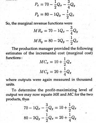
Q_x = 80 — 8P_X + 6 Py Q_y= 40-4P_y + 4P_X;

where the outputs were measured in thousand units and the prices in rupees per unit. Solving these two forecasted demand functions simultaneously, the corresponding inverse demand functions are ob­tained:

If we solve these equations simultaneously, we would obtain the profit-maximizing output levels: Q_X = 30 (i.e., 30,000 units) and Q_Y = 20 (i.e., 20,000 units). Finally, using these outputs in the inverse demand functions, the profit-maximizing price for X was found to be Rs. 40 and for Y Rs. 45.

Thus, the basic point to note is that if a firm produces products that are related in consumption, profit maximization requires that output levels and prices be determined jointly. To be more specif­ic, in a joint-product firm, the profit-maximizing price for a particular commodity will be deter­mined not only by its own demand and cost condi­tions but also by those of the related products.

---

6. Multiple Products that are Complements in Production:

We may now consider a firm that produces products that are complements in production.

For simplicity, we consider the case of a firm that produces the two products in fixed propor­tions. The classic example of this is that of mutton and hides. Clearly, these are joint products that are complements in production. Moreover, this joint production of the two products is characterized by fixed proportions — for each additional unit of mutton (say, 40 kg.) produced, one additional hide will be produced.

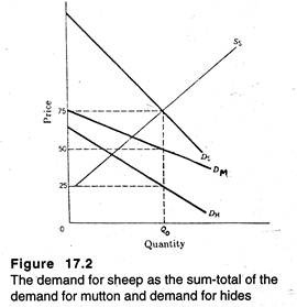
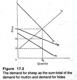
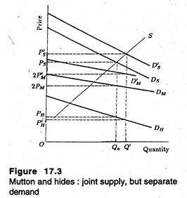
We may consider, for example, the fact that one sheep produces one hide and two sides of mutton. In Figure 17.2, we show the demand curves for pairs of sides’ of mutton and for hides, which are labeled D_M and D_H, respectively.

The price that buyers are willing to pay for a sheep is equal to the sum-total of what people are ready to pay for the components parts. Thus, the demand curve for sheep D_S is equal to vertical summation of the demand curve for hides and the demand curve for pairs of sides of mutton.

If the market for sheep is competitive, market equilibrium will occur where the demand curve for sheep intersects its supply curve. This is shown in Figure 17.3 at output of OQ₀ sheep. The price of a sheep (Rs. 75) is equal to the price of a hide (Rs. 25) plus twice the price of a side of mutton (Rs. 50).

Such instance of joint production characterized by fixed proportion can easily be multiplied. In- deed, petroleum refining industry has similar char­acteristics.

With an existing refinery and the pre­vailing mix of input crude oils, production of an ad­ditional barrel of one of the lighter distillates, such as gasoline, would necessitate the production of some additional amount of the heavier distil­lates, like fuel oil.

We continue to assume that the firm produces only two products, X and Y. Thus, our problem is to determine the level of production and the price for each of these complementary products.

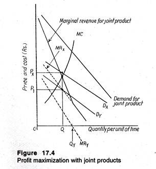
In Figure 17.4, we illustrate the problem graph­ically. The demand curves for the two products are D_x and D_y and the corresponding marginal revenue curves are MR_X and MR_y. The marginal cost curve is shown as the marginal cost of producing the joint product.

In order to determine how much of the joint product is to be produced, we have to derive the de­mand curve and the marginal revenue curve for the joint product. The joint product demand curve is de­rived by summing up the individual demand curves vertically. For example, given some level of pro­duction of mutton and hides, the total price re­ceived is equal to the sum of the prices received for the two products.

The marginal revenue curve for the joint product is also arrived at by vertical addition of MR_X and MR_y, with one major difference. In Figure 17.4, MR_y becomes zero at an output Q_y. If commodity Y is sold in excess of Q_y, the marginal revenue of Y would be negative. It is quite obvious that the maximum amount of Y the firm will sell is Q_y.

Therefore, the marginal revenue curve for the joint product is the vertical sum of MR_X and MR_y until MR_y is zero. For outputs beyond the Q_y level, only commodity X would be produced and sold, so the joint marginal revenue curve will coincide with MR_X. As a result we obtain the “kinked” joint product marginal rev­enue curve of Figure 17.4.

The profit-maximizing level of output is deter­mined by equating the joint marginal revenue to the joint marginal cost. In Figure 17.4, this implies that the firm will produce Q units of the joint prod­uct. The firm will then sell Q units of X at a price of P_x and Q units of Y at a price of P_y.

To see how the firm can implement profit- maximization with joint products, as analysed above, we may consider the following example.

Example 3:

Profit Maximization with Joint Products:

ICI produces refined chemicals. In one of its di­visions it produces joint product, i.e., as it refines the raw chemical input, the processes will yield equal amounts of two products X and Y. In other words, the two products are produced in fixed pro­portions. The question faced by the marketing man­ager is how much of products X and Y to sell and at what prices?

The demand functions for the two products had been forecasted as:

Qx = 285-P_x; Q_y = 150-2P_y

where the outputs are measured in thousand kgs and the prices in Rs. per kg. The marginal revenue curves corresponding to these demand functions are

MR_X. = 285-2Qr; MR_y=75-Q_y

Here, the marginal revenue function for Y is equal to zero at an output of 75 (i.e., 75,000 kg). Thus, for output levels of the joint product before or equal to 75, the marginal revenue function for the joint product is the vertical summation of the two marginal revenues.

MR = 360 – 3Q

For output levels above Q = 75, the joint product marginal revenue function would coincide with MR_X.

Given the existing stock of capital, it has been estimated that the incremental (marginal) cost function for refining the chemical input to be

MC= 10+ 2Q

where marginal cost is measured in Rs. per kg. and output (Q) is in thousand kgs.

By equating marginal revenue and marginal cost for the joint products, we get

360 – 3Q = 10 + 2Q

The profit-maximizing level of production of the joint product is Q = 70 (i.e., 70,000 kg.). Using Q = 70 in two demand curves, the marketing manager would find that the firm should sell 70,000 kg. of X at Rs. 2.15 per kg. and 70,000 kg. of Y at Rs. 0.40 per kg.

So long we have analysed the situation where the firm will produce and sell the two products in fixed proportions. This may not always happen.

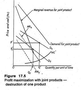
A different type of situation is shown in Figure 17.5. The only difference between this figure and Figure 17.4 is the location of the marginal cost curve for the joint product. In such a situation, the firm will produce Q’ units of the joint product. Moreover, since MR_X is positive at Q’, the firm will sell Q’ units of X at the price P’_x. But at Q’, MR_y is negative.

So the firm will sell only Q_y units of Y at the price of P_y and must destroy the remainder (i.e., Q’ – Q_y units). The reason is not far to seek. If these units are marketed, the firm’s revenues will fall.

Example 4:

Profit Maximization with Joint Products:

Let us have a fresh look at the decision faced by the marketing manager of ICI. Suppose that a new estimate of the incremental (marginal) cost of re­fining the joint product is made and the following result is obtained:

MC= 80 + 1/2 Q

Again, by equating this marginal cost function to the joint product marginal revenue function of our previous example, we get:

360 – 3Q = 80 + 1/2Q

The implied optimal output be Q = 80. Howev­er, the marketing manager knows quite well that, at this production level, the marginal revenue for product Y would be negative. Thus, for this range of production, the joint product marginal revenue func­tion coincides with MR_X; so, to determine optimal production, marginal cost has to be equated to the marginal revenue for product X.

285 – 2Q = 80 + 1/2 Q

Thus, in this situation, the optimal output of the joint product is Q = 82. In other words, the firm will produce 82,000 kg of chemicals X and Y.

Since MR_X is positive at Q = 82, the firm will sell the 82,000 kg of X and charge a price of Rs. 2.03 per kg, as is seen from the demand function.

However, ICI will sell chemical Y only to that point at which its marginal revenue is zero. The implication is that since MR_Y = 0 when Q = 75, the firm will sell only 75,000 kg of chemical Y and will destroy the remaining 7,000 kg. From the demand function for Y, the price that will be charged for the 75,000 kg of Y that is sold is 37.5 paise per kg.

---

7. Multiple Products that are Substitutes in Production:

We may now consider a different situation – a situation in which the multi-product firm produces products which are substitutes in production. This situation is likely to occur in the case of a firm that produces several models of the same basic product, such as different models of electronic watches.

These different models do compete for the limited production facilities and common resources of the firm. Thus, they are substitutes in the production process of the firm.

In the long run, the firm can make appropriate adjustment in its production fa­cility in order to produce the profit-maximizing level of each product. But in the short run, the firm suffers from capacity constraints and has to deter­mine how to allocate its limited production capaci­ty among the competing products in order to maxi­mize profit.

Thus, the short-run case is one of constrained op­timization. The firm has to maximize profit subject to the constraint imposed by the limited production facility. Let us suppose the firm produces only two product, X and Y, by using its existing production fa­cility, and that the cost of operating this facility does not vary with the product produced.

The mar­ginal benefit derived by producing an additional unit of either product is the marginal revenue that would be generated. For product X, this is MR_X. The marginal cost of producing an additional unit of one product is the fall in output of the competing prod­uct. Thus, the relevant concept for decision-making is the opportunity cost concept.

For product X, the marginal cost is the corresponding reduction in the production of Y, i.e., ∆Y. By contrast, the marginal cost of producing an additional unit of Y is ∆X. A firm will maximize its objective function subject to a constraint when the ratios of marginal benefit to marginal cost are equal for all decision variables.

In this context, the implication is that profit will be maximized when the levels of production of the two products are such that

MR_X/∆Y = MR_Y/∆X

To see how this happens in practice, we may con­sider a simple example.

Example 5:

The Allocation of Assembly Line Time:

Suppose, a company produces two products, X and Y, which are unrelated in consumption but are substitutes in production. For example, Prentice Hall of India (PHI) may print two books — Dean’s Managerial Economics (product X) and Basu’s Consti­tutional Law (product Y), from the same press. No student requires both the titles at the same time.

So they are unrelated in consumption. But since they are printed from the same press, they are substi­tutes in production. Since these two products are produced on the assembly line, they compete for the limited time available. The question facing the production manager of PHI is : How should an eight-hour production day be allocated between the production of X and the production of Y?

The demand functions for the two products were estimated to be

Q_x= 60 – ½ P _x; Q_y = 40-2/3 P_y

where the quantities were the number of units de­manded per day and the prices were expressed in rupees per unit. From these estimated demand func­tions, the marginal revenue functions were

MR_X = 120-4Q_x; MR_y = 60-3Q_y

Consultation with the plant engineers indicated that, in one hour of production time, either two units of X or four units of Y could be produced. In a sense, the “production functions” for the two prod­ucts are

Q_X = 2H_X; Q_y = 4H_y

where H_x and H_y denote, respectively, one hour of assembly line time in the production of X and Y. Thus, the marginal cost of using an additional hour in the production of X is ∆Y = 4. That is, if that plant utilizes an additional hour for the product X, it must sacrifice the production of four units of Y. Likewise, the marginal cost of an additional hour in the production of Y is ∆X = 2.

Therefore, the firm will maximize profit subject to the limitation of the eight-hour production day if it produces amounts of X and Y such that the fol­lowing condition is satisfied:

120 – 4Q_x/4 = 60-3Q_y/2

This condition requires that Q_x = (3/2)Q_y. Using the “production functions” above, this profit- maximization condition (2/3) Q_y may be rewritten in terms of hours devoted to the production of the two products as

H_x — 3H_y.

For profit maximization, the firm has to devote assembly line time to X and Y in the ratio of 3:1.

If we use this optimality condition with the time constraint (i.e., H_x + H_y = 8), it is clear that, to maximize profits, six hours will be devoted to product X and two hours to product Y. That means that PHI will produce 12 units of X per day and 8 units of Y; so, the optimal prices are Rs. 96 per unit for X and Rs. 48 per unit for Y.

There is an alternative way of expressing the optimization condition for the allocation of the production facility between the production of X and Y. Let F denote the level of usage of the production facility.

Then ∆X/∆F and ∆Y/AF are the marginal product of the production facility in the production of X and Y, respectively. Then, dividing both sides of the previous condition by AF, we derive the fol­lowing optimization condition:

(MR_X) x (MP_F/X) = (MR_y) x (MP_Fy) or MRP_X = MRPy.

Or

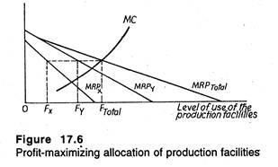
If, over an extended period of time, the firm en­joys sufficient flexibility and is able to vary its us­age of its production facilities, we can generalize this condition. In Figure 17.6, the horizontal axis measures the level of usage of the limited produc­tion facilities. However, the analysis is slightly different from the previous one in the sense that we consider a single marginal cost curve.

It is because we assume that costs depend only on the level of us­age of the production facility and have no relation to the type of product produced.

Profit will be max­imized at the point at which marginal cost is equal to total marginal revenue product. Thus, the usage level of the production facility will be F total- The problem faced by the production manager is: how this level of usage (e.g., machine hours) is to be di­vided between the two products?

It is quite obvious that if the allocations were such that MRP_X > MRP_y, profit could be increased by reallocating from the production of Y to the pro­duction of X. This would reduce MRP_X and raise MRP_y.

Such a reallocation would continue until the marginal revenue products are equal, i.e., MRP_X = MRP_y. Furthermore, since the total marginal reve­nue product curve is simply the sum of the two indi­vidual curves, the profit-maximizing condition boils down to:

MRP_TOTAL = MC = MRP_X = MRP_y.

The implication is that profits will be maximized when production is allocated in such a way that the marginal additions to revenue are the same for the two products. The following example bears rel­evance in this context.

Example 6:

Optimum Utilization of Multi-Purpose Plants:

The production manager of ABC Inc., wanted to consider changing the daily production schedule for the plant producing X and Y from the present 8 hour-daily schedule.

That is, the production man­ager was interested in knowing two things:

(1) What was the optimal level of usage (hours of op­eration) of the plant?

(2) How should this level of usage be allocated between the production of the two products?

Using the demand forecasts of the marketing department and the estimates of the “production functions” prepared by the plant engineer, esti­mates/forecasts of the marginal revenue product of the production facility in the production of X and Y were

MRP_X = [120 – 4 (2H_X)] x (2) = 240 – 16H_X

MRP_Y = [60 – 3(4H_X)] x 4 = 240 – 48 H_Y.

By summing these two curves horizontally, the to­tal marginal revenue production function was ob­tained, i.e., these functions were inverted to find H_X and H_Y, then the hours were summed (H Total – H_X + H_Y). The resulting total MRP was

MRP Total = 240 – 12 H_TOTAL.

Let us suppose that the plant supervisor arrived at the following estimate of the additional cost of op­erating the plant an additional hour – the incre­mental (marginal) cost for usage of the plant

MC = 72+ 2H.

By equating the total marginal revenue product of an hour’s usage of the plant with the marginal costs of an additional hour’s usage, we get:

240 – 12H = 72 + 2H.

Thus, the production manager of ABC Inc. found that the optimal level of usage of the plant was 12 hours per day. At this level of usage, MRP Total = MC = Rs. 96. To allocate these hours between the production of X and Y, the marginal revenue prod­ucts for the production facility in the production of X and Y will both have to be equal to 96:

240 – 16Hx = 96; 240 – 48H_y = 96.

Thus, the optimal allocation would be 9 hours in the production of X and 3 hours in the production of Y.

---

8. Cost of Multiple Products:

Most modern companies produce a number of products by losing certain common resources. So there is the problem of allocating certain costs among dif­ferent products. There are certain costs which are traceable to individual products, e.g., purchased parts and components.

In such cases the problem of cost allocation does not arise. However, there are certain costs which are common to several products, i.e., they cannot be easily identified with a single product. An obvious example of this is the cost of the factory building. All multi-product firms face the problem of identifying parts of common costs with individual products.

Another point to note is that there are certain costs which remain unchanged at all levels of out­put. In such cases we cannot measure or quantify in­cremental cost and the question of cost allocation is not very relevant. What has to be allocated is short-run variable cost. In other words, the real problem faced by management is allocation of vari­able common costs.

Accounting Allocations of Product Costs:

In accounting, the general practice is to allocate joint costs on the basis of the assumption that joint (multiple) products are produced in fixed propor­tion.

The two most frequently used methods for such allocation of common costs among individual prod­ucts are:

(1) Physical measure,

(2) Sales value.

1. Physical Measure:

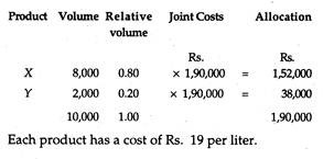
This method of cost allocation utilize some physical attribute common to all joint products to allocate joint costs to individual products. The most frequently used attributes are: weight, volume, surface area, and potential or actual heat content. Under this method the common attribute is summed and the joint costs are allocated on the basis of each product’s relative portion of it.

This proce­dure is really meaningful when there is a close re­lationship between the physical measure and the selling price of individual products. However, Joel Dean has argued that “the most widely used meth­od of allocation of common costs is some measure of direct labour costs.”

Example 1:

Using liters as a measure, Lakme allocates the following joint costs of X and Y:

2. Sales Value:

Irrespective of the relationship between physi­cal measures and selling prices, the use of relative sales values as a basis for allocating joint costs makes enormous good sense. At least this procedure avoids misleading inferences. This method is based on the assumption that a pro rata recovery of joint costs is made in each rupee of sales revenue, with­out distinction among the different products.

The allocated costs of each product bears an exact pro­portional relationship to its selling price. Howev­er, this method has one major drawback: it is uncer­tain and hence has no usefulness in product line problems, since it hardly provides any basis for comparing costs with revenues.

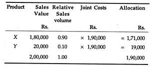
Example 2:

Assuming that selling prices for X and Y are Rs. 22.50 and Rs. 10.00 per liter, respectively, Lakme allocates the following joint costs to X and Y:

Product X costs Rs. 21.375 per liter (i.e., Rs. 1,71,000 + 8,000) and product Y costs Rs. 9.50 per liter (i.e., Rs. 19,000 + 2,000).

In the short run, it is very difficult to vary the product-mix. So we retain our assumption of joint products produced in fixed proportions. In the case- of such products, separate product costs are indeter­minate. For instance, it is difficult to think of the separate costs of producing pineapple and pineap­ple juice because one unavoidably accompanies the other. This is a case of joint products.

As Joel Dean has noted, “When an increase in the production of one product causes an increase in the output of an­other product, then the products and their costs are traditionally defined as joint.” By contrast, when one product is much less important than the other, it is called a by-product, such as sugar and khand- sari. Usually a by-product is produced by utilizing a waste material.

If the increase in the output of one product does not require an increase in the output of another, it is possible to determine separate incremental costs. On the contrary, when an increase in the production of one commodity requires a sacrifice or reduction of the output of the other, the concept of opportunity cost bears much relevance.

For example, the princi­pal cost of canning pineapples is the foregone op­portunity to pack pineapple juice. These are called alternative products.

The important point to note is that it is always possible to compute the cost of an alternative prod­uct in terms of the foregone profits from the other product. On the other hand, the cost of a joint prod­uct (as distinguished from the cost of the product range) is largely and essentially indeterminate.

It is virtually impossible to allocate cost when joint products are produced in fixed proportions. It is be­cause there is no alternative but to produce the package. No cost is variable and hence avoidable. However, in the case of products produced in varia­ble proportions, marginal costs with respect to changes in output-mix prove to be useful in deciding between alternative product-mixes.

---

9. Allocate Cost Among Multiple Products:

Statistical analysis enables us to isolate the common variable costs as a function of aggregate output and then to allocate these costs among mul­tiple products by using various alternative meth­ods.

Joel Dean has suggested four such methods:

1. Prima facie, “when there is a traceable ele­ment of cost which in the aggregate is highly correlated with output and/or with the vari­able common costs to be allocated”, then vari­able overheads may be prorated on the basis of a single input, e.g., direct labour hours. This method of allocation gives a fairly good approximation to normal marginal cost for in­dividual products.

2. Secondly, all variable overheads can be allo­cated to individual products on the basis of the relative mix of the product’s total of traceable costs — e.g., the sum of direct labour and direct materials.

3. Thirdly, cost accountants follow the practice of allocating each variable overhead separ­ately, selecting from a range of “traceable in­puts the one that appeared to be most closely related. For example, electric power might be allocated on the basis of machine hours, in­ventory expenses on the basis of direct materi­als, and indirect labour on the basis of direct labour.”

4. Finally, cost allocation may be made, through statistical analysis, by finding “how each element of overhead cost varies with each of several dimensions of output and use these relationships as the basis for allocating the variable portions of each element of over­head cost, separately to individual products on the basis of their dimensional characteris­tics. … For instance, in a furniture factory, cer­tain clerical and stockroom costs vary with the number of production orders, and spoilage may depend on the number of new styles.”

Job Scheduling:

A major problem that arises in a factory is known as job scheduling or job sequencing. When out­put is produced in batches there is the problem of securing the best possible use of the machines and equipment available. The demand for the service of a machine varies from one batch to another but any machine is available for only one job at a time.

This implies that another job is kept waiting until the machine is free. This is often observed in the printing industry. Sometimes, however, a machine is kept idle for a different reason because the next job is still being processed on another machine. The situation is continually varying in accordance with the orders placed in any planning period.

The following three situations may be consid­ered:

1. Different products may require the same pro­cess in the same sequence but for different time periods.

2. Each job has its own sequence of processes, again with different time requirements.

3. Each job needs a range of processes but the se­quence is not rigidly determined and fol­lowed, that A can be done before C, or C can be done before A.

Further, complication crops up because in some production situations the processing time of one job may be affected by preceding or following jobs.

Johnson’s Rule:

We often make use of Johnson’s rule if there are only two machines or processes through which a number of jobs have to be passed in the same se­quence.

The procedure has the following six-step sequence:

1. First, one has to tabulate the processing times by jobs and processes.

2. Then, from the table, one has to select the shortest operational time. If there is a tie, an arbitrary choice has to be made.

3. If the minimum time relates to the first oper­ation, one has to put the job at the beginning of the sequence.

4. If the minimum time relates to the second op­eration one must put the job at the end of the sequence.

5. Then one has to delete the job from the table and look for the next shortest operation.

6. Finally, one must repeat the process until all jobs are placed.

We consider the following table to illustrate the concept. It is an example of the processing times required by each of five jobs on two machines:

Here the shortest operational time is for the second operation of job A, e.g., 2 hours. Following step 4 above, we put job A last in the sequence and ignore it altogether. In the remaining four jobs, the next shortest time is for job E.

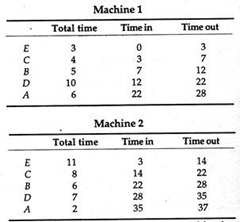
Since this is the first operation, we have to place E at the beginning of the sequence. The next lowest job is job C, once again in the first operation, so we put C after E. Finally, we arrive at the sequence E, C, B, D, A. We may now arrange the sequence in the following table.

We can see that the total time covered by the completed operation in 37 hours during which Ma­chine 1 is remaining idle for 9 hours and Machine 2 for 3 hours, assuming that no other job is available at present to utilise the machines fully.

---