Cost-Minimising with Changing Output Levels (With Diagram)

Let us make an in-depth study of the cost-minimising with changing output levels.

We have already seen how a cost-minimising firm selects a combination of inputs to produce a given level of output.

Now we analyse to see how the firm’s costs depend on its output level.

So we have to see, for each output level, the firm’s cost-minimising input quantities and then calculate the resulting cost.

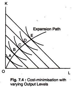
The cost-minimising exercise can be performed for every output that the firm is considering to produce. Fig. 7.4 shows a result of this analysis. Each of the points A, B, C, D and E represents a point of tangency between an isoquant and an isocost.

The curve, which moves upward to the right from the origin, and traces the points of tangency, is the expansion path of the firm which illustrates the least cost combinations to produce each level of output in the long-run when both inputs can be varied.

The expansion path gives information about the total cost of all variable inputs as the output changes. It tells us the lowest long-run total cost of producing each level of output.