International Trade under Varying Opportunity Cost Conditions | Economics

We shall analyse below the international trade between two countries under varying opportunity cost conditions.

Constant Opportunity Cost and International Trade:

When production is governed by constant returns to scale, the marginal rate of transformation between two commodities, say X and Y, remains constant and the opportunity cost curve or transformation curve is a falling straight line. In such a case the relative cost of producing the commodities remains unchanged, irrespective of the ratio in which they are demanded.

If the slopes of transformation curves in two countries are the same, so that the opportunity cost curves are parallel to each other, no trade can be possible. The gains from trade can emerge only when the slopes of the transformation curves are different. It signifies the presence of differences in relative cost ratios. These two cases have been explained through Figs. 6.2 (a) and 6.2 (b).

In Fig. 6.2 (a), AB and A₁B₁ represent the opportunity cost curves concerning the countries A and B respectively. These two straight line opportunity cost curves are parallel. Therefore, their slopes are exactly equal. The slope of AB is OA/OB and that of A₁B₁ is OA₁/OB₁ and OA/OB = OA₁/OB₁.

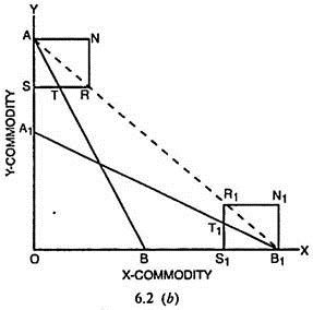
In such a case, the cost ratios of two commodities in both the countries are also equal. Therefore, international trade cannot take place as no country stands to gain through trade.

If there are comparative cost differences, the slopes of the production possibility curves will be different as shown in Fig. 6.2 (b). AB is the production possibility curve of country A and A₁B₁ is the production possibility curve of country B. The slopes of these curves clearly show that country A has a comparative advantage in the production of Y over country B. The latter has the comparative advantage over A in the production of commodity X.

There will be specialisation by A in Y and B in X. They will exchange commodities in the ratio indicated by the dotted price line AB₁. Suppose country A wants to consume quantities of two commodities indicated by R. Country A will export AS = NR quantity of Y and import SR = AN quantity of X. Country B wants to consume the quantities of two commodities indicated by R₁. She will export B₁S₁ = R₁N₁ quantity of X and import R₁S₁ = B₁N₁ quantity of Y.

The production possibility curve AB shows that AS quantity of Y can be exchanged for ST quantity of X in the domestic market. But the international trade permits the exchange of AS quantity of Y for SR quantity of X so that gain from trade for country A amounts to TR (= SR – ST) quantity of X. In case of country B, B₁S₁ quantity of X can be exchanged for S₁T₁ quantity of Y in the domestic market. The international trade, however, permits the exchange of B₁S₁ of X for R₁S₁ quantity of Y. The gain from trade for country B will be R₁T₁ (= R₁S₁ – S₁T₁) quantity of Y.

If both the countries are of equal size, there will be complete specialisation in both the countries. If one of the countries is large and the other is small, there will be complete specialisation in the latter. The former will have only partial specialisation. In such a situation, the larger gain from trade will be available to the smaller of the two countries.

Increasing Opportunity Cost and International Trade:

The production under constant returns to scale can be possible, when it is assumed that there are fixed factor proportions and that factors of production have equal efficiency in producing relative outputs of two commodities. In actual life, factor specificity, lack of perfect substitution and varied efficiency of factor units in different lines of production lead to decreasing returns to scale and the opportunity cost may go on increasing. The international trade in such a situation is explained through Figs. 6.3 (a) and 6.3 (b).

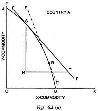
In Fig. 6.3 (a), AB is the production possibility curve for country A. Under the decreasing returns to scale, it is concave to the origin. EE is the domestic price ratio line before trade takes place. It is tangent to the production possibility curve AB at R. After the commencement of trade, when international exchange ratio represented by line FF is given, the equilibrium is determined by the tangency between AB and FF at S.

Country A specialises in the production of Y. If the point of consumption in A is T, this country will export SN quantity of Y to import NT quantity of X. The consumption point T will lie on a higher community indifference curve than the point R before the commencement of trade. So country A will enhance her welfare through trade.

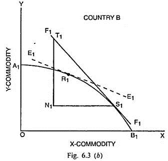
In Fig. 6.3 (b), A₁B₁ is the production possibility curve for country B. Before international trade, the domestic price ratio line E₁E₁ is tangent to A₁B₁ at R. When trade commences, the equilibrium is determined through the tangency between A₁B₁ and line F₁F₁ which represents international exchange ratio at S₁. Country B specialises in the production of X as it has comparative advantage in the production of this commodity.

If the point of consumption is T₁, country B will export N₁S₁ quantity of X and import N₁T₁ quantity of Y and be at a higher level of satisfaction T₁ than in the pre- trade situation R₁. When equilibrium situation is achieved for both the countries, the export of Y commodity SN equals the import of this commodity N₁T₁ and the export of X commodity N₁S₁ equals the import of this commodity NT.

In the situation of increasing costs, the countries will probably not specialize completely because the increased production may result in a loss of comparative advantage vis-a-vis the other country. To quote H. Robert Heller, “Countries experiencing increasing cost of production will specialize in the production of the commodity in which they enjoy a comparative advantage. The specialization need not be complete.”

Decreasing Opportunity Cost and International Trade:

If the production of both the commodities in the two countries is governed by increasing returns to scale, the production possibility curve or transformation curve in both the countries will be convex to the origin. The international trade in such a situation can be explained through Fig. 6.4.

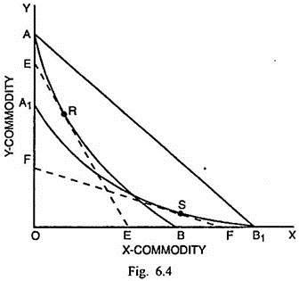
AB is the production possibility curve for country A and A₁B₁ is the production possibility curve for country B. In the absence of international trade, the production equilibrium of country A is determined at R where the domestic exchange ratio indicated by price line EE becomes equal to the MRT_xy. Similarly the tangency between A₁B₁ and domestic price line FF for country B determines the production equilibrium point at S.

If the international trade commences, the international exchange ratio is indicated by the price line AB₁. The position of opportunity cost curve AB and greater steepness of domestic price line EE relative to international exchange ratio line AB₁ shows that country A will specialise completely in the production of Y commodity.

On the opposite position of curve A₁B₁ and relatively greater steepness of AB₁ than FF indicates that country B will specialise completely in the production of X commodity. Country A will export Y commodity and import X commodity. Country B, on the opposite, will export X commodity to import Y commodity.

The point of consumption equilibrium for both the countries, determined by the tangency between commodity indifference curve and international exchange ratio line, will lie somewhere on the international exchange ratio line AB₁. Such a point will indicate a higher level of satisfaction than either at R or S, signifying the gains from trade to both the countries.

Increasing and Decreasing Opportunity Cost and International Trade:

PC. Kindelberger has discussed another possibility of trade equilibrium where the transformation curve is neither uniformly convex nor uniformly concave to the origin. One segment of it may be convex and the other may be concave. Such a possibility arises if one of the products is a primary product, such as cotton, the production of which is governed by diminishing returns to scale or increasing opportunity cost.

The other commodity is a manufactured one, such as steel, the production of which is governed by increasing returns to scale or decreasing opportunity cost. Fig. 6.5 takes the case of two such commodities Y and X. The production of Y is governed by decreasing returns to scale whereas that of X is governed by increasing returns to scale. AL, the upper stretch of opportunity cost curve AB is concave to the origin while LB, the lower stretch of opportunity cost curve is convex to the origin. L is the point of inflexion.

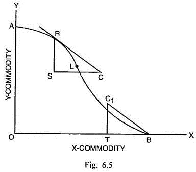
Given the international exchange as denoted by the line RC, the production equilibrium is determined at R which lies on the concave stretch of the opportunity cost curve AB and there is only partial specialisation in the production of Y. If C is the consumption equilibrium point, there will be export of RS of Y in exchange of SC quantity of X commodity. If the production of Y is stretched beyond the point of inflexion L, we enter the zone of increasing returns.

Now given the international price line BC₁ which is parallel to RC, the production equilibrium is determined at B and there is complete specialization in the production of commodity X. If consumption equilibrium point is C₁, the country will export BT quantity of X and in return import C₁T quantity of Y. Such a shift from L to B or from increasing cost to decreasing cost product is not, however, easy in the face of free competition. At least temporarily, the country will have to raise tariffs against the import of Y from abroad for encouraging the domestic production of X- commodity.

Criticisms of the Opportunity Cost Theory:

Haberler’s reformulation of the classical comparative cost theory in terms of opportunity costs has been acclaimed widely as a much more exact, precise and scientific explanation of the patterns of trade than the real cost approach. It is definite advance over the real cost approach.

The opportunity cost theory has distinct merits over the Ricardian real cost approach. First, it abandoned the labour theory of value and attempted to build up the production and trade model on the more realistic assumption of two or more factors of production. Second, the Ricardian comparative costs theory analysed trade under the conditions of constant costs alone.

The opportunity cost theory, on the other hand, stresses that the trade can be possible, no matter whether the costs are constant, increasing or decreasing. In fact, the opportunity cost theory demonstrated the validity of comparative costs principle under varying costs.

Third, this theory provided theoretical framework for analyzing the general equilibrium or trade equilibrium in the much more simple way than that adopted by Jacob Viner. Fourth, this theory draws attention, in an effective manner, towards the issue of factor substitution. It is a significant departure from the earlier analysis concerning production and international trade.

Jacob Viner has mounted scathing criticism of the opportunity cost theory.

His main objections against this theory are as follows:

(i) Welfare Consideration:

Viner held that the opportunity cost approach was inferior to the real cost approach from the viewpoint of welfare. According to him, the principle of opportunity cost failed to measure real costs in terms of strain, sacrifice or disutility. However, this criticism is not valid. If the opportunity cost curve can show the gain from trade for the trading countries, it cannot be condemned on the ground of neglect of welfare. Haberler asserted that the real cost approach, based on unreal and dubious hypothesis, on the contrary, was devoid of explanatory value and was of little use for determining the welfare function.

In his words, “The theory cannot be useful for welfare analysis unless it also has some explanatory value. If its explanatory value is limited in the sense that it describes only tendencies and holds only approximately (except under ideal conditions), then the same limitations apply to the welfare implications. And if it can be entirely dispensed with as an explanatory device, the same must be true, one should think, in the welfare field.”

The modern writers like Kemp, Samuelson and Baldwin have successfully analysed the gains from trade in terms of welfare through the device of production possibility curve and utility possibility curves. Even Jacob Viner, the staunch supporter of the traditional theory, has recognized the analytical superiority of the opportunity cost theory.

(ii) Neglect of Change in Factor Supplies:

Jacob Viner attacked the opportunity cost theory also on the ground that it neglected the changes in the factor supplies. V.C. Walsh demonstrated that the changes in factor supplies can be measured in terms of opportunity costs by involving changes in commodity price ratio and marginal productivities of factors.

(iii) Neglect of Leisure:

Another objection raised by Jacob Viner against the opportunity cost approach was that it failed to take into account the preference for leisure vis-a-vis income. Walsh rebutted even this objection. According to him, when the trading countries exchange goods at an international price ratio, there is normally an increase in real income part of which may be in the form of more leisure. Walsh proved his point through the use of a three-dimensional figure. About that attempt Richard Caves commented. Walsh’s argument demonstrates that…the transformation curve defined for fixed quantities of factor inputs will change in both shape and size when the preference for leisure varies.

(iv) Unrealistic Assumptions:

The opportunity cost approach rests upon several unrealistic and invalid assumptions like fixed factor supplies, absence of external economies or diseconomies and the existence of perfect competition in the product as well as factor markets. These assumptions do not hold valid in the real life. These theoretical deficiencies greatly reduce the analytical significance of this approach.

Even if we recognise these defects, yet it scores over the real cost approach by a decisive margin. In this context, Samuelson observes, “Without pursuing this matter further, I would still say that the simplifications made in the (unqualified) opportunity- cost approach are empirically much less absurd than those resorted to by any other real-cost or pain-cost doctrine; the opportunity cost approach is more fertile because it can be readily extended into a general equilibrium system and it is used even by those who in principle, attack it.”