Haberler’s Opportunity Cost Theory (With Assumptions) | Economics

In this article we will discuss about the Haberler’s opportunity cost theory.

Gottfried Haberler has attempted to restate the comparative costs in terms of opportunity cost. He demonstrates that the doctrine of comparative costs can hold valid even if the labour theory of value is discarded. The theory determines the cost of producing a commodity in terms of the alternative production that has to be foregone for producing the commodity in question.

Elaborating upon the opportunity cost, Haberler writes that “the marginal cost of a given quantity X of a commodity A must be regarded as that quantity of commodity B which must be foregone in order that X, instead of (X-1) units of A can be produced. The exchange ratio on the market between A and B must equal their costs in this sense of the terms.”

The opportunity cost is what has been given up in order to have some quantity of another thing. If an additional unit of one commodity has to be produced, the productive resources are to be diverted from the production of some other commodity to the given commodity.

The resultant decrease in the quantity of the second commodity represents the opportunity cost of the additional quantity of the given commodity. For instance, if India has to reduce the production of cotton by 2 lakh bales in order to raise the production of wheat by 1 lakh tons, then the opportunity cost of one unit of wheat is two units of cotton (1W = 2C).

Haberler made use of opportunity cost curve to express the opportunity cost of one commodity in terms of the other. The opportunity cost curve has been called as the ‘transformation curve’ or ‘production possibility curve’ by Paul Samuelson and ‘ production frontier’ or ‘production indifference curve’ by A.P. Lerner.

Assumptions of Haberler’s Opportunity Cost Theory:

Haberler’s opportunity cost theory rests upon the following main assumptions:

(i) The economic system is in a state of full employment equilibrium.

(ii) There is perfect competition in commodity and factor markets.

(iii) Price of each commodity equals the marginal cost of producing it.

(iv) Price of each factor equals its marginal productivity.

(v) The supply of factors is fixed.

(vi) The state of technology is given.

(vii) There are two trading countries A and B.

(viii) Each country produces two commodities, say X and Y.

(ix) Each country has two productive factors- capital and labour.

(x) There is perfect factor mobility within each country.

(xi) The factors of production are perfectly immobile between the two countries.

(xii) Neither of the two countries imposes any restrictions upon international trade.

On the basis of the above assumptions, it is possible to determine the opportunity cost curve or the production possibility curve of any country.

The production possibility curve indicates different combinations of two commodities that a country can produce with the given factor endowments and technology. The slope of the production possibility curve is determined by the ratio of units of the commodity given up in order to have one unit of the other commodity. This ratio is termed as a marginal rate of transformation (MRT).

If two commodities X and Y are being produced by a country and some quantities of labour, capital and other inputs are diverted from the production of Y to the production of X, the additional production of X involves the sacrifice of some quantity of Y. In other words, certain units of Y given up have been transformed into the marginal unit of X. The rate at which marginal unit of X is being substituted for certain units of Y is called the marginal rate of transformation.

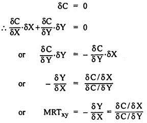
Alternatively, the MRT_xy can be defined as a ratio of the marginal cost of X to the marginal cost of Y.

This can be derived as below:

Here δC stands for change in total cost, δC/δX and δC/δY are the marginal costs of X and Y commodities respectively.

Assuming infinitesimally small changes in X and Y, δC will be equal to zero.

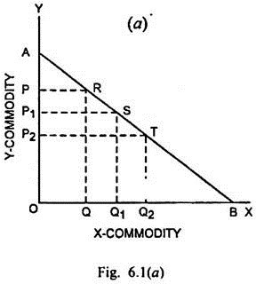
Since the MRT_xy is negative, the opportunity cost curve or transformation curve slopes down from left to right. The opportunity cost curve may be a straight line, convex to the origin or concave to the origin, depending on whether return to scale in a country is constant, increasing or decreasing respectively.

At every point on the straight-line opportunity cost curve AB in Fig. 6.1 (a) the MRT_xy remains equal, MRTxy = – δY/δX = PP₁/OQ₁ = P₁P₂/Q₁Q₂. It also signifies that marginal costs of X and Y remains unchanged and production of both the commodities is governed by constant returns to scale or constant opportunity cost. It implies that all factors of production are equally efficient in all lines of production. Since this is not true in real life, the production possibility curve is not likely to be a falling straight line.

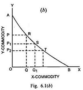
In Fig. 6.1 (b), the opportunity cost curve AB is a falling convex towards the origin, MRT_xy in this case goes on decreasing.

(PP₁/QQ₁ > P₁P₂/Q₁Q₂)

This happens when production is governed by increasing returns to scale or the cost of X in terms Y goes on diminishing as less and less units of Y are given up in order to have more units of X. Even this situation is not realistic because larger production of X will cause reduced significance of X for the commodity in terms of the commodity Y. This figure, on the opposite, indicates increasing marginal significance of X.

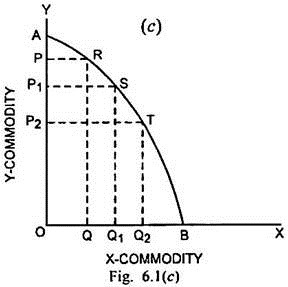
In Fig. 6.1 (c), the opportunity cost curve AB is a falling concave curve towards the origin. In this case, MRT_xy goes on increasing (PP₁/QQ₁ < P₁P₂/Q₁Q₂).

The opportunity cost curve assumes this slope, when production is governed by diminishing returns to scale. As there is an increase in the production of X commodity, MC of X rises while that of Y decreases. This case seems to be more realistic because in this situation, a greater availability of X commodity shows a decreasing significance of this commodity in terms of units of Y commodity.