
J.E. Meade assembled the analytical devices like the production possibility curve, the community indifference curves and offer curves in order to explain the general equilibrium of production, consumption and trade involving the two trading countries. Fig. 4.17 is employed to explain the general equilibrium situation concerning the two trading countries A and B.
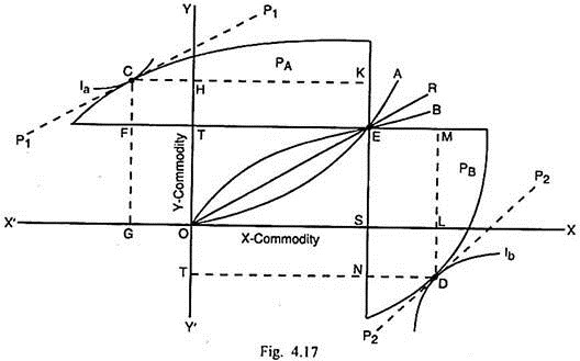
In Fig. 4.17, the commodity X is measured along the horizontal scale X’OX and the commodity Y is measured along the vertical scale YOY’. OA and OB are the offer curves of the two countries A and B respectively. These curves cut each other at E. This is the equilibrium exchange point and the international price ratio between two commodities X and Y is measured by the slope of the international exchange ratio line OR. In equilibrium, country A exports OS quantity of X and imports ES quantity of Y.
PA is the production block of country A and PB is the production block of country B. Both have their origin at the point E. Ia is the community indifference curve of country A. The domestic price ratio line P1P1 of country A is tangent to Ia and the production possibility curve at this country at C.
ADVERTISEMENTS:
So C is the point of consumption and production equilibrium of this country. Production of X commodity is CK and its consumption is CH so that the quantity of X left for export is HK (= OS). Production of Y commodity in country A is CF but its consumption is CG so that the demand for FG (= ES) quantity of Y commodity is met through import.
Ib is the community indifference curve of country B. The domestic price ratio line P2P2 related to country B is tangent to lb and the production possibility curve of this country at D. This is the point of production and consumption equilibrium of this country. The production of X commodity is DN but its consumption is DT so that the excess demand NT is met through imports from country A.
Country B produces DM quantity of Y commodity, out of which DL quantity is consumed at home and the remaining quantity LM is meant for export. Thus in the position of equilibrium, exports of country B are LM (= ES) quantity of Y and imports are NT (= OS).
Fig. 4.17 shows that both the countries are simultaneously in the position of consumption, production and trade equilibrium. In the position of general equilibrium, there is not only a proper balance between their respective exports and imports, but also an equality of the domestic price ratio of X and Y with the international price ratio of two commodities.
ADVERTISEMENTS:
This is evident from the fact that P1P1 and P2P2 the domestic price ratio lines or exchange ratio lines of countries A and B have exactly the same slope as the international exchange ratio line OR (P1P1 ॥ P2P2॥ OR). As a result of the consumption, production and trade equilibrium, both the countries move to their respective highest possible community indifference curves as well as the highest production frontiers. This reflects the gain from international trade for both the countries.