
In this article we will discuss about trade equilibrium in terms of community indifference curves and offer curves.
Trade Equilibrium in Terms of Community Indifference Curves:
In a closed economy, the general equilibrium is determined, when the production and consumption sectors are both in equilibrium. The equilibrium in the consumption sector takes place if the marginal rate of substitution of one commodity, say X, for the other commodity, say Y, becomes equal to the price ratio of those two commodities (MRSxy = Px/Py). The equilibrium in the production sector is possible when the marginal rate of transformation between these two commodities become equal to their price ratio (MRTxy = Px/Py).
So the condition of the equilibrium of the whole system gets satisfied when:
MRSXy = MRTXy = PXPy
ADVERTISEMENTS:
In the position of equilibrium, the slope of some commodity indifference curve will be exactly equal to the slope of the production possibility curve or the transformation curve. Such a situation can be shown through Fig. 4.9.
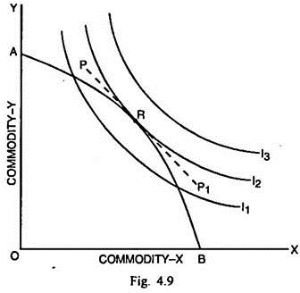
In Fig. 4.9, commodity X is measured along the horizontal scale and commodity Y is measured along the vertical scale. I1, I2 and I3 show the map of community indifference curves. AB is the production possibility curve. The line PP1 measures the domestic price ratio of X and Y commodities. The consumption equilibrium is determined at R when MRSxy = Px/Py or the slope of community indifference curve I2 is exactly equal to the slope of the price line.
The community neither wants to buy more nor less units of any of the two commodities. The production equilibrium is also determined at R where the price line PP1 is tangent to the production possibility curve AB. At this point MRTxy is equal to the price ratio of X and Y (MRTxy = Px/Py) and there is neither a rise nor a fall in the production of either of the two commodities. Thus R is the point of general equilibrium, where the price line is simultaneously tangent to both the community indifference curve and the production possibility curve and MRSxy = MRTxy = Px/Py.
ADVERTISEMENTS:
In an open economic system, the consumption and production equilibrium situations are not coincidental but the international trade brings about adjustments between production and demand in the case of each trading nation. In the final equilibrium problem, the value of exports becomes exactly equal to the value of imports. The general equilibrium of the given country in the post-trade situation can be explained through Fig. 4.10.

In Fig. 4.10, commodity X is measured along the horizontal scale and commodity Y along the vertical scale. I1, I2 and I3 are the community indifference curves. PP1 is the domestic price ratio line. AB is the production possibility curve or the opportunity cost curve. Before trade, the consumption and production equilibrium is determined at R where OQ of X + ON of Y is produced and consumed by the country. If trade takes place and P2P3 is the international exchange ratio line, the production equilibrium is determined at S by the tangency between P2P3 and opportunity cost curve AB.
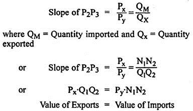
Hence MRTxy = Px/Py. The consumption equilibrium is determined by the tangency of P2P3 with the higher community indifference curve at T where MRSxy = Px/Py. At point S, this country produces OQ1 quantity of X and consumes OQ2 of it. The excess supply Q1Q2 is exported. At T, the demand for Y commodity is ON2 but domestic production of this commodity is only ON1 so that it will import N1N2 quantity of it. It is possible to show that in such a situation of equilibrium after trade, the value of exports is equal to the value of imports.
Trade Equilibrium in Terms of Trade Indifference Curves:
A trade indifference curve corresponds to each community indifference curve of a country. As a result, each country has its respective map of trade indifference curves. It is the objective of each trading country to reach its highest possible trade indifference curve. The trade equilibrium will take place where there is tangency between the international price ratio line and the trade indifference curves of the two countries. It is explained through Fig. 4.15.
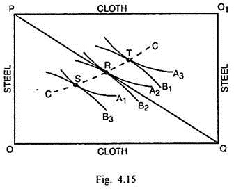
Fig. 4.15 is an Edgeworth type box diagram. Fig. with origin at O is concerned with the country A and inverted Fig. with origin as O1 is related to country B. Commodity cloth is exportable of A and importable of B, while steel is exportable of B and importable of A. The curves A1, A2 and A3 represent trade indifference map of country A. B1, B2 and B3 curves represent the trade indifference map of country B. These curves are tangent at S, R and T. Joining these points, the curve CC can be drawn which is the contract curve.
All the points on the contract curve represent such combinations of two commodities at which the exchange may take place. If PQ is the international exchange ratio line or price ratio line, it cuts the contract curve at R where the trade indifference curve A2 of country A and B2 of country B become tangent to each other. This point represents the optimum position from the point of view of both the countries and each one of them is better off through trade.
Trade Equilibrium in Terms of Offer Curves:
The offer curve of a particular country shows different quantities of her exportable commodity, which she offers to another country for importing certain quantities of the importable commodity. Given the offer curves of two trading countries, the trade equilibrium is determined, where there is intersection of these offer curves. It is explained with the help of Fig. 4.16.
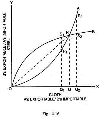
In Fig. 4.16, OA is the offer curve of country A and OB is the offer curve of country B. Cloth is exportable commodity of country A. It is importable commodity of country B. Steel is the exportable commodity of country B and importable commodity of country A. At point R1 on the offer curve OA, the country A is willing to export OQ1 quantity of cloth in exchange of R1Q1 quantity of steel. Country B, however, is willing to export S1Q1 quantity of steel is order to import OQ1 quantity of cloth.
At point R2, country A is prepared to export OQ2 quantity of cloth in exchange of R2Q2 quantity of steel. But country B is willing to give up only S2Q2 of steel for OQ2 quantity of cloth. Therefore, exchange cannot take place in either of the two situations.
ADVERTISEMENTS:
The equilibrium takes place at point R, where the offer curves OA and OB intersect each other and OQ quantity of cloth is exchanged for RQ quantity of steel between the two trading countries. The line joining O and R is the international exchange ratio line. The slope of the line OR is measured by the ratio of quantity imported to the quantity exported (RQ/OQ).