Two-Country Trade Equilibrium | International Trade | Economics

In two-country trade equilibrium model it is supposed that there are two countries A and B and they produce two commodities— X and Y.

The trade equilibrium of these countries can be analysed under constant, increasing and decreasing cost conditions as below:

1. Trade Equilibrium under Constant Costs:

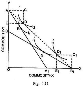
In this case it is supposed that both countries A and B are producing at the constant costs so that their opportunity cost curves are negatively sloping straight lines. This is the classical Smith-Ricardo type case. It may be explained through Fig. 4.11.

In Fig. 4.11, AA₁ and BB₁ are the production possibility curves or opportunity cost curves of countries A and B respectively. Since the production in both countries is governed by constant costs, the slopes of opportunity cost curves remain unchanged and these are negatively sloping straight lines. I₁ and I₂ are the community indifference curves of country A whereas I₁^’ and I₂‘ are the community indifference curves of country B. In autarky (absence of trade), the consumption and production equilibrium of A occurs at R and that of B takes place at S because of the tangency between their respective opportunity cost curves and indifference curves.

If trade takes place, country A specialises in the production of Y as it has comparative cost advantage in the production of Y. Country B specialises in the production of X, as it possesses comparative cost advantage in the case of this commodity. Their respective comparative cost advantages or specialisations are evident from the differences in the slopes of their opportunity cost curves. Since there is complete specialisation, the points of production for countries A and B are respectively A and B₁.

By joining these points, the international exchange ratio line AB₁ can be drawn. It is tangent to indifference curve I₂ of country A and indifference curve I₂‘ of country B. Therefore, D is the point of consumption equilibrium of A and D₁ is the point of consumption equilibrium of B. Country A exports AE (= CD) quantity of Y. It is equal to imports of country B, which are D₁E₁ (= C₁B₁). The imports of country A are DE (= AC). These are equal to exports of country B, which are B₁E₁ (= C₁D₁).

Thus exports of each country are just sufficient to pay for her imports and there is equilibrium in respect of demand and supply in both the countries. In addition, the trade shifts consumption equilibrium in both the countries to their higher community indifference curves. That is a measure of gain from trade for both the countries.

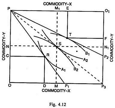
The trade equilibrium under constant cost conditions can be explained also with the help of Edgeworth’s Box Diagram. It is supposed that there are two countries A and B. In the absence of trade, each one of them produces both the commodities X and Y. According to Fig. 4.12, the Fig. with origin as O is concerned with country A and that with origin O₁ is concerned with country B. PP₁ is the opportunity cost curve of country A and PP₂ is that of country B. Since both the countries are producing under constant cost conditions, these opportunity can curves are negatively sloping straight lines.

A₁ and A₂ are the community indifference curves of country A. B₁ and B₂ are the community indifference curves of country B. In the absence of trade, the consumption and production equilibrium in country A is determined at R where the opportunity cost curve PP₁ (which is the domestic exchange ratio lines of country A) becomes tangent to the indifference curve A. This country produces and consumes CR quantity of X and RD quantity of Y respectively. Similarly the point T is the consumption and production equilibrium point for country B. At this point the opportunity cost curve PP₂ is tangent to indifference curve B₁ of this country. At T, country B produces and consumes TF quantity of X and ET quantity of Y.

If trade commences, country A will specialise completely in the production of Y and country B will specialise completely in the production of X commodity. PP₃ represents the international exchange ratio line for them. Given PP₃, the higher community indifference curve A₂ of country A has tangency with the international exchange ratio line at S. At this point, country A consumes SM quantity of Y and SN quantity of X.

The international exchange ratio line PP₃ is also tangent to the community indifference curve B₂ of country B at S. Thus S is the point of trade equilibrium for both the countries. At this point, country B consumes SN₁ quantity of X and SM₁ quantity of Y. Country A which specialises in the production of Y will consume SM quantity of it herself and the remaining output SM₁ of it is exported to country B.

At the same time, country B, which specialises in the production of X commodity, consumes SN₁ quantity of it herself and the remaining quantity SN is exported to country A. Thus country A exports SM₁ quantity of Y to B and imports SN quantity of X from that country. This exchange results in gain for both the countries, as both of them are better off after the commencement of trade and each one of them shifts to her higher community indifference curve.

2. Trade Equilibrium under Increasing Costs:

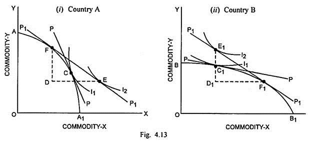
The production under the conditions of constant costs is only a special case which may not exist in real life. Eventually the law of diminishing returns or increasing costs becomes applicable in almost all the fields of production. Since the cost ratio tends to rise, the opportunity cost curves or production possibility curves pertaining to the trading countries are negatively sloping concave curves to the origin. The trade equilibrium related to two countries under the conditions of increasing costs is explained through Fig. 4.13.

In Fig. 4.13, X-community is measured along horizontal scale and Y-community is measured along the vertical scale. Fig. 4.13 (i) is concerned with country A and Fig. 4.13 (ii) is concerned with country B. AA₁ is the production frontier or opportunity cost curve of country A and BB₁ is the production frontier of country B.

In Fig. 4.13 (i), C is the point of consumption and production equilibrium of country A in the absence of trade because it is the point of tangency between the community indifference curve I₁ and domestic exchange ratio line PP and also the point of tangency between the opportunity curve AA₁ and the exchange ratio line PP. If trade commences, this country will specialise in the production of Y commodity. This is evident from the slope of AA₁.

Given the international exchange ratio line P₁P₁, the production equilibrium in this country gets determined at F where P₁P₁ is tangent to AA₁. The consumption equilibrium is determined at E where P₁P₁ is tangent to the higher community indifference curve I₂ of county A. This country will export FD quantity of Y to country B and import DE quantity of X-community from that country.

In Fig. 4.13 (ii), C₁ is the point of consumption and production equilibrium of country B in the absence of trade. At this point, domestic exchange ratio line PP is tangent to both the production possibility curve BB₁ and the community indifference curve I₁. If trade commences, this country will decide to specialise in the production of X-community. This is evident from the slope of the opportunity cost curve BB₁ of this country.

The international exchange ratio line P₁P₁ is tangent to BB₁ at F₁ which is the point of production equilibrium and it is tangent to higher community indifference curve I₁ at E₁ which is the point of consumption equilibrium. Since the consumption equilibrium in both the countries shifts to their respective higher indifference curves, both derive gain from trade. Country B exports D₁F₁ (=DE) quantity of X-commodity to country A. At the same time, B imports D₁E₁ (=DF) quantity of Y-commodity from the country A.

3. Trade Equilibrium under Decreasing Costs:

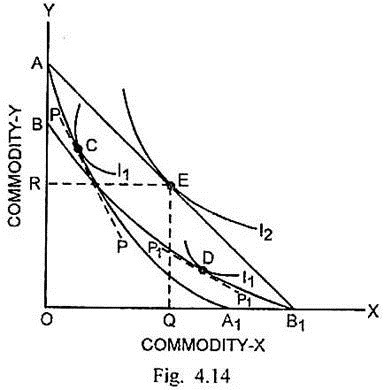
If the production is governed by increasing returns to scale or decreasing costs, the production possibility curve is a negatively sloping convex curve to the origin. The trade equilibrium concerning two countries A and B can be explained with the help of Fig. 4.14.

In Fig. 4.14, the two countries produce under the conditions of increasing returns or decreasing costs so that their opportunity cost curves are negatively sloping convex curves to the origin. Given their different factors endowments, AA₁ is the opportunity cost curve of country A and BB₁ is the opportunity cost curve of country B.

In the absence of trade, the consumption and production equilibrium of country A is determined at C where its domestic exchange ratio line PP is tangent to both AA₁ and the community, difference curve I₁. The production and consumption equilibrium of country B is determined at D where the domestic exchange ratio line P₁P₁ of this country is tangent to its opportunity cost curve as well as its community indifference curve I₁.

If trade commences, country A will specialise completely in the production of Y commodity and B will specialise completely in the production of X commodity. This is on account of their respective comparative cost advantages and decreasing costs. The international exchange ratio line is AB₁. The production equilibrium of country A is determined at the point A, which is the maximum limit of production of Y commodity. For country B, the production equilibrium is at B₁, the maximum limit of production of this commodity by country B.

Assuming identical tastes in the two countries, the consumption equilibrium of the both is determined through the tangency of international exchange ratio line AB₁ and the commodity indifference curve I₂. Each country consumes OQ of X commodity and OR of Y commodity.

Country A exports AR quantity of Y to country B and imports RE (= OQ) quantity of X from it. Country B, on the other hand, exports B₁Q (= RE) quantity of X-commodity to country A and imports EQ (= AR) quantity of Y- commodity from it. This exchange ensures gain from trade for the both because their consumption equilibrium shifts to the higher community indifference curve I₂ reflecting greater welfare for each one of them.