Revealed Preference Theory (RPT) (With Diagram)

In this article we will discuss about the Revealed Preference Theory (RPT) put forth by prof. Samuelson.

The Concept of Revealed Preference:

Prof. Samuelson has invented an alternative approach to the theory of consumer behaviour which, in principle, does not require the consumer to supply any information about himself.

If his tastes do not change, this theory, known as the Revealed Preference Theory (RPT), permits us to find out all we need to know just by observing his market behaviour, by seeing what he buys at different prices, assuming that his acquisitions and buying experiences do not change his preference patterns or his purchase desires.

Given enough such information, it is even theo­retically possible to reconstruct the consumer’s indifference map.

Samuelson’s RPT is based on a rather simple idea. A consumer will decide to buy some particular combination of items either because he likes it more than the other combinations that are available to him or because it happens to be cheap. Let us suppose, we observe that of two collections of goods offered for sale, the consumer chooses to buy A, but not B.

We are then not in a position to conclude that he prefers A to B, for it is also possible that he buys A, because A is the cheaper collection, and he actually would have been happier if he got B. But price information may be able to remove this uncertainty.

If their price tags tell us that A is not cheaper than B (or, B is no-more expensive than A), then there is only one plausible explanation of the consumer’s choice—he bought A because he liked it better.

More generally, if a consumer buys some collection of goods, A, rather than any of the alternative collections B, C and D and if it turns out that none of the latter collections is more expensive than A, then we say that A has been revealed preferred to the combinations B, C and D or that B, C and D have been revealed inferior to A.

Therefore, if the consumer buys the combination E₁ (x₁, y₁)of the goods X and Y and does not buy the combination E₂(x₂, y₂) at the prices (p¹_x, p¹_y,) of the goods, then we would be able to say that he prefers combination E₁ to combination E₂, if we obtain

The complete set of combinations of the goods X and Y to which a particular combination is revealed preferred can be found with the aid of the consumer’s price line. Let us suppose that the consumer’s budget line is L₁M₁ in Fig. 6.104 and he is observed to purchase the combina­tion E₁ (x₁, y₁) that lies on this line.

Now, since the costs of all the combinations that lie on the budget line are the same as that of E₁ and since the costs of all the combinations that lie below and to the left of the budget line are lower than that of E₁ we may say that E₁ is revealed preferred to all the combinations lying on or below the consumer’s budget line.

Again, since the costs of the combinations that lie above and to the right of the budget line are higher than that of E₁ we cannot say that the consumer prefers E₁ to these combinations when he is ob­served to buy E₁, because here E₁ is the cheaper combination.

We have to note here the difference between “preference” and “revealed preference”. Com­bination A is “preferred” to B implies that the consumer ranks A ahead of B.

But A is “revealed preferred to B” means A is chosen when B is affordable (no-more-expensive). In our model of consumer behaviour, we generally assume that people are choosing the best combination they can afford that the choices they make are preferred to the choices that they could have made. That is, if (x₁ y₁) is directly revealed preferred to (x₂, y₂), then (x₁, y₁) is, in fact, preferred to (x₂, y₂).

Let us now state the RP principle more formally:

Let us suppose, the consumer is buying the combination (x₁, y₁) at the price set (p’_x, P’_y) let us also suppose that another combination is (x₂, y₂), such that p’x₁ + p’_yy₁ ≥ p’_xx₂ + p’_yy₂. Now, if the consumer buys the most preferred combination subject to his budget constraint, then we will say the combination (x₁, y₁) is strictly preferred to combination (x₂, y₂).

The Assumptions:

With the help of the simple principle of RP, we may build up a powerful theory of consumer demand. The assumptions that we shall make here are:

(i) The consumer buys and uses only two goods (X and Y). The quantities x and y of these goods are continuous variables.

(ii) Both these goods are of MIB (more-is-better) type. This assumption is also known as the assumption of monotonicity. This assumption implies that the ICs of the consumer are nega­tively sloped.

(iii) The consumer’s preferences are strictly convex. This assumption implies that the ICs of the consumer would be convex to the origin, which again implies that there would be obtained only one point (the point of tangency) on the budget line of the consumer that would be chosen by him over all other affordable combinations.

This assumption is very important. On the basis of this assumption, we shall obtain a one- to-one relation between the consumer’s price-income situation or budget line and his equilib­rium choice—for any particular budget line of the consumer, there would be obtained one and only one equilibrium combination of goods and for any combination to be an equilibrium one, there would be obtained one and only one budget line.

(iv) The fourth assumption of the RP theory is known as the weak axiom of RP (WARP). Here we assume that if the consumer chooses the combination E₁(x₁, y₁) over another afford­able combination E₂(x₂, y₂) in a particular price-income situation, then under no circumstances would he choose E₂ over E₁ if E₁ is affordable.

In other words, if a combination E₁ is revealed preferred to E₂, then, under no circumstances, E₂ can be revealed preferred to E₁.

(v) The fifth assumption of the RP theory is known as the strong axiom of RP (SARP). According to this assumption, if the consumer, under different price-income situations, reveals the combination E₁ as preferred to E₂, E₂ to E₃,…, E_k-1 to E_k, then E₁ would be revealed preferred to E_k and E_k would never (under no price-income situation) be revealed preferred to E₁.

Revealed Preference—Direct and Indirect:

If RP is confined to only two combinations of goods, E₁ and E₂, and if, in a particular price- income situation, E₁ (x₁,y₁) is revealed preferred to combination E₂ (x₂, y₂), then it is said that E₁ is directly revealed preferred to E₂.

But if preferences are considered for more than two combinations and if preferences are established by way of transitivity of RP, then it is a case of indirectly revealed preference. For example, if E₁ is revealed preferred to E₂,…, E_k-1 to E_k, then by SARP, we say E₁ is indirectly revealed preferred to E_k.

Violation of the WARP:

Let us consider Fig. 6.105. Here let us suppose that, under the price income situation represented by the budget line L₁M₁, the consumer purchases the combination E₁ (x₁, y₁) and he reveals combination E₁ (x₁ y₁) as preferred to E₂ (x₂, y₂).

For here he chooses E₁ over the affordable combination E₂. Again, let us suppose that when the budget line of the consumer changes from L₁M₁ to L₂M₂, the consumer buys the combination E₂ (x₂, y₂), although he could have obtained the affordable combination E₁ (x₁, y₁), i.e., under L₂M₂, E₂ is revealed preferred to E₁.

What we have seen here is that under the budget line, L₁M₁, the combination E₁ is revealed preferred to E₂ and under a different budget line L₂M₂, E₂ is revealed preferred to E₁. Obviously, the consumer here violates the WARP.

The reason for this violation may be that the consumer here does not attempt to obtain the most preferred combination subject to his budget constraint; or, it may be that his taste or some other element in his economic environment has changed which should have remained unchanged by our assumptions.

Now, whatever may be the reason for the violation of WARP, this violation is not consistent with the model of consumer behaviour that we are discussing.

The model assumes that the consumer wants to maximise his level of satisfaction and, that is why, when he chooses a particular combination, say, E₁ subject to his budget, that must be the most ‘preferred’ to all other affordable combinations, and none of these ‘other’ com­binations can be ‘preferred’ to E₁ under a different budget. WARP puts emphasis on this simple but important point. We may give the formal statement of WARP in the following way.

If a particular combination E₁ (x₁ y₁) is directly revealed by the consumer as preferred to a different combination E₂ (x₂, y₂), then E₂ would never be revealed by the consumer as preferred to E₁.

In other words, if the consumer is observed to purchase E₁ (x₁, y₁) at the price set (p_x⁽¹⁾, p_y⁽¹⁾) and E₂ (x₂ , y₂) at the price set (p_x⁽¹⁾, p_y⁽²⁾), then if (6.138) below holds, then (6.139) must never hold:

As we have seen, WARP has been violated in Fig. 6.105, when the consumer buys combination E₁ on L₁M₁ and E₂ on L₂M₂. Here the preference ordering of the consumer breaks down. It may be verified in Fig. 6.105 that the IC tangent to L₁M₁ at E₁ and the IC tangent to L₂M₂ at E₂ cannot be non-intersecting in this case.

In Fig. 6.106, on the other hand, let us suppose, the consumer buys the combination E₁ on L₁M₁ and the combination E₂ on L₂M₂. Here when he buys E₁ he chooses E₁ over the affordable combination E₂, i.e., E₁ is revealed preferred to E₂. But when he buys E₂, he chooses E₂ over an unaffordable E₁, i.e., E₂ is not revealed preferred to E₁.

Therefore, here, WARP is not violated, and so, here the preference ordering of the consumer does not break down. It may be seen in Fig. 6.106 that the IC tangent to L₁M₁ at E₁ and the IC tangent to L₂M₂ at E₂ would be non- intersecting.

Significance of the SARP:

Let us now discuss the significance of the strong axiom of revealed preference (SARP). According to this axiom, if the consumer reveals a combination E₁ (x₁, y₁) as preferred to another combination E₂ (x₂, y₂) and if E₂ (x₂, y₂) is revealed preferred to E₃ (x₃, y₃) then E, would always be revealed preferred to E₃.

This may be called the transitivity of revealed preferences. Now, if the consumer is a utility-maximising one, then the transitivity of revealed preferences would lead to transitivity of preferences—if E₁ is preferred to E₂ and E₂ to E₃, then E₁ would be preferred to E₃.

But this is necessary to ensure that the ICs are non-intersecting and the non-interesting ICs are necessary for arriving at the utility-maximising solution. It is evident that if any of the WARP and SARP is violated, then utility-maximisation cannot be achieved by the consumer.

Revealed Preference Theory and the Slutsky Theorem:

Let us now see how the RPT can be used to prove the Slutsky Theorem which states that if the income effect (IE) for a commodity is ignored, then its demand curve must have a negative slope. To explain this, we shall take the help of Fig. 6.107.

In this figure, let E₁ (x₁, y₁) represent the combination of goods that the consumer initially purchases when his budget line is L₁M₁. We want to show here that a ceteris paribus fall in the price of good X from L₁M₁ will increase the purchase of the good if we ignore the income effect, i.e., if we consider only the substitution effect (SE).

Let us suppose that the imaginary budget line for Slutsky-SE is L₂M₂. This line will be flatter than L₁M₁, since the price of X has fallen, ceteris paribus, and this line (L₂M₂) will pass through the combination E, so that, as per the Slutsky condition, the consumer might be able to buy the initial combination, if he liked, under the changed circumstances.

Let us now see, because of the SE, the point the consumer may select on the imaginary budget line L₂M₂ (if it is to be different from E), would be a point like E₂ to the right of the point E₁. To prove that this must be so, we have to note that selection of any point on L₂M₂ such as E₃ which lies to the left of E₁, is ruled out by WARP.

This is because, initially, E₁ has been revealed preferred to E₃, since E₃ lies below L₁M₁. But if E₃ were chosen when the price line was L₂M₂, it (E₃) is revealed preferred to E₁ since E₁ is no-more-expensive than E₃ (for they both lie on the same budget line L₂M₂). In that case, we obtain that E₁ is revealed preferred to E₃, and vice versa, which violates WARP.

Thus no point on L₂M₂ which, like E₃, lies to the left of E₁, can be chosen. On the other hand, if the consumer chooses a point like E₂ on L₂M₂ to the right of E₁, then there is no harm to the weak axiom, because when he purchases E₂, E₂ is revealed preferred to the no-more-expensive combination E₁ but, initially, when he purchased E₁ (on L₁M₁) and not a point like E₂, he did this, because E₁ was cheaper than these points.

From the analysis, it is clear that the SE of a fall in the price of X will generally increase the demand for the relatively cheaper commodity X at a point like E₂ to the right of E₁. Thus, the Slutsky theorem is deduced from the revealed preference approach.

We have seen that if the price of X falls, ceteris paribus, and if the income effect of this price fall is ignored, then the SE would increase the demand for X, i.e., the demand curve for X would be negatively sloped, and the law of demand is obtained.

From Revealed Preference to Preference:

The principle of revealed preference (RP) is rather simple, but at the same time it is very powerful. Supported by the assumptions we have made, the RPT enables us to obtain the con­sumer’s preference pattern or indifference curves (ICs) from his revealed preferences.

No in­trospective data are required from the consumer to achieve this task. If we know the price- income situation of the consumer as represented by his budget line and his point of revealed preference on the line, we would be able to derive his IC that passes through this point. The process of obtaining the IC is described below.

Let us suppose that the budget line of the consumer is L₁M₁ in Fig. 6.108 and the combina­tion of the goods that the consumer is observed to purchase, is E₁ (x₁, y₁). As we know, the consumer here prefers the point E, directly to all other points on the budget line or in the area OL₁M₁. For, in spite of all these points being within his budget, he purchases E₁. “All these points” are considered to be “worse” than E₁.

On the other hand, the costs of all the combinations lying to the right of the budget line L₁M₁ are more than that of the point E₁, or, E₁ is cheaper than these points. Apparently, the consumer chooses E₁ over these points because they are more expensive, and we cannot say anything about the ‘revealed’ preference of E₁ to any of these points.

That is why, the area in the commodity space to the right of L₁M₁ is known as the area of ignorance. We shall see, however, with the help of the assumptions of the RPT, that some of the points in the area of ignorance are directly or indirectly preferred or inferior to E₁ and some of the points are indif­ferent with E₁.

These latter points that are indifferent with E₁ give us the indifference curve (IC) passing through E₁, Let us now see how we can derive this curve.

At the very first, let us consider the area K₁E₁B₁. The commodity combinations (except E₁) belonging to this area are directly preferable to the consumer to E₁ , since all these combinations have more of either one or both of the goods than the point E₁. These combina­tions may be called the “better” combinations.

So far we have obtained that the consumer directly prefers E₁ to the points to the left of the budget line L₁M₁, i.e., those lying in the area OL₁M₁ and he directly prefers the points lying in the area K₁E₁B₁ to E₁. Therefore, his IC through the point E₁ if it is obtained, would be spread in the space between these two areas, and it would touch the line L₁M₁ and the area K₁E₁B₁ at the point E₁.

Let us now consider the points in the area of ignorance lying above the line L₁M₁ and outside the area K₁E₁B₁. At first, we shall try to identify the points that the consumer prefers less to E₁—these points may be called the “worse” points. In order to do this, let us consider any point E₂ lying on L₁M₁ to the right of E₁.

Let us suppose that the consumer is observed to purchase E₂ when his budget line is L₂M₂. He, therefore, reveals the point E₂ as preferred to the points to the left of the budget line L₂M₂. Since E₁ has already been revealed preferred to E₂, the consumer prefers E₁ to all these points lying in the area OL₂M₂.

Since a portion of this area, viz., □OL₂E₂M₁ belongs to the area OL₁M₁, here the net increase in the area of “worse” points is obtained to be □E₂M₁M₂. The consumer prefers E₁ indirectly to the points of this area through the combination E₂—he prefers E₁ to E₂ and E₂ to these points.

We may again increase the area of “worse” points to the right of E₁ by considering any other point E₃ lying on the line L₁M₁ to the right of E₂. Let as suppose that the consumer purchases E₃ when the budget line is L₃M₃. That is, he reveals the point E₃ as preferred to the points lying in the area OL₃M₃.

Again, since E₁ has already been revealed preferred to E₃, he may be said to prefer E₁ to these points in the area OL₃M₃. Here the net increase in the area of points worse than E₁ has been □SM₂M₃. The consumer prefers E₁ indirectly (through the point E₃) to the points in □SM₂M₃.

So far we have seen how we may lessen the area of ignorance by considering the points on the budget line L₁M₁ to the right of E₁. We may also do this job by considering points on L₁M₁ to the left of E₁. Let us suppose, E₄ is any point on L₁M₁ to the left of E₁ and the consumer is observed to purchase E₄ when his budget line is L₄M₄.

The point E₄, therefore, is revealed preferred to the points lying in the area OL₄M₄. But the point E₁ has already been revealed preferred to point E₄ and so the consumer prefers E₁ to these points. Here, if we leave out the common portion of areas OL₁M₁ and OL₄M₄, we obtain that the consumer indirectly prefers E₁ to the points of □E₄L₁L₄.

Therefore, now we have been able to reduce the area of ignorance by □E₄L₁L₄. We may, in this way, go on reducing the area of ignorance by considering more points on L₁M₁ lying to the left of the point E₁.

So far we have reduced the area of ignorance by increasing the area of “worse” combinations. We may now see how we may increase the area of “better” combinations outside the area K₁E₁B₁ and thereby reduce further the area of ignorance. Let us suppose that the consumer is observed to purchases the point E₅ when his budget line is G₁E₁H₁.

Here the consumer will prefer all the points in the area K₂E₅B₂ to the point E₅, since these points have more of either one or both the goods. Also it is now revealed that the consumer prefers E₅ to E₁, for he chooses E₅ over the affordable E₁. Therefore, what we obtain here is that the points lying in the area K₂E₅B₂ are “better” than the point E₁.

Here, if we leave out the portion of □K₂E₅B₂ which is in common with □K₁E₁B₁, we find that there has been a net increase in the area of “better” points and net decrease in the area of ignorance—this net increase is represented by the area lying in between the lines K₂E₅, K₁T and E₅T.

Again, because of our assumptions of convex preference and MIB, the consumer will prefer the points in □E₁E₅T to E₁. Therefore, this area is also added to the area of “better” combinations and the area of ignorance is reduced accordingly. We may go on increasing the area of “better” combinations in this way. For example, the consumer is observed to purchase the point E₆ on the budget line G₂ E₁ H₂.

Here we would find that the area of the “better” points gets an increase by the area in between the lines RB₁ RE₆ andE₆B₃ plus the area E₁E₆R. Therefore, these areas are also added to the area of “better” combinations and the area of ignorance is reduced accordingly.

In Fig. 6.108, we have seen that on the basis of the idea of revealed preference and with the help of the assumptions made, we may go on increasing the area of the combinations that are “worse” than a particular combination E₁ from below and we may also go on increasing the area of the combinations that are “better” than E₁ from above.

In the limit, the area between these two areas would get reduced to a border line curve of indifference. By applying the advanced methods of calculus and also intuitively, we may obtain that this indifference curve of the consumer would pass through the point E₁, would lie in between the two paths like K₂E₅E₁E₆B₃ and L₄E₄E,E₂SM₃ and would be convex to the origin.

We have seen how we may obtain a consumer’s IC through any particular combination E₁. Applying the same process, we may obtain his IC through any other point in the commodity space, i.e., we would obtain his indifference map.

Let us now see with the help of Fig. 6.109, how we may conclude intuitively that the borderline between the areas of “bet­ter” and “worse” combinations than any point E₁ is an IC through that point.

In Fig. 6.109, we have represented that the areas of better and worse combinations than E₁ have been made to advance towards each other and in the limit the gap between them looks like an IC, and actually, it would be an IC, passing through E₁ We can understand this in the following way.

Let us move vertically from one point to another in the commodity space of Fig. 6.109 starting from any point like N, (x°, y₁) of the area of worse combinations. As we move upwards vertically, the quantity of good X remains the same at x₀ and that of good Y increases, and ultimately, very near the border of the “worse” area we shall arrive at a point like N₂ (x°, y₂).

Let us suppose, if we still move upwards slightly beyond N₂, we shall arrive at a point N₃ (x°, y₃) in the area of “better” combi­nations. Now we may easily understand intuitively that there lies a point N* (x₀, y*), y₂ < y* < y₃, in the infinitesimally small vertical gap between the points N₂ and N₃ which is neither worse nor better than E₁ but which is indifferent with E₁.

Therefore, if we join the points E₁ and the points like N* by a curve we would obtain the required IC through E₁.

Indifference Curve, Revealed Preference and Cost of Living Index:

Let us first consider two price index formulas. One is Laspeyre’s formula and the other is Paasche’s formula. Laspeyre’s price index number is the ratio of two aggregates—aggregate of current year prices at base year quantities and that of base year prices at base year quantities. Let us suppose that an individual purchases two goods.

The base year and current year prices of the goods are p₀₁, p₀₂ and p_t1, p_t2. Also the base year and current year quantities of the goods purchased by the consumer are q₀₁, q₀₂ and q_t1, q_t2. Then Laspeyre’s price index would be

Here the base year quantities of the goods have been taken as weights of their prices. L gives us the price index in the current year if the base year price index is 1. For example, if L = 1.5, then we obtain that current year price index is 1.5 when the base year price index is 1, i.e., the prices in the current year are 50 per cent more than those in the base year.

Laspeyer’s price index may be interpreted in another way. The numerator of the right hand side of (6.140) gives us the cost of the base year basket of goods (q₀₁ , q₀₂) at the current year prices (p_t1, p_t2), and the denominator gives us the cost of buying the same basket of goods at the base year prices (p₀₁, p₀₂).

Looking in this way, L = 1.5 gives us that the cost of buying the base year basket of goods has increased by 50 per cent in the current year over the base year. That is, the Laspeyre’s price index number L may also be considered as the Laspeyre’s cost of living index number.

Let us now come to Paasche’s price index number which is the ratio of the aggregate of current year prices at current year quantities and that of the base year prices at current year quantities. Therefore, we obtain Paasche’s price index number as

Here the current year quantities of the goods have been taken as the weights of their prices. Just like the Laspeyre’s price index number, Paasche’s price index number may also be consid­ered as the Paasche’s cost of living index number. It gives us the percentage increase in the cost of buying the current year basket of goods in the current year over the base year.

Let us now come to the total expenditure of the consumer in the base year and in the current year. In the base year his total expenditure is, say, E₀, and he purchases the quantities q₀₁ and q₀₂ at prices p₀₁ and p₀₂. Therefore, his budget line in the base year is

E₀ = p₀₁q₀₁ +p₀₂q₀₂                    (6.142)

Similarly, in the current year his total expenditure is, say, E_t, and he purchases the quantities q_tI and q_t2 at the prices p_t1 and p_t2. Therefore, his budget line in the current year is

E_t = p_t1q_t1 + p_t2q_t2                       (6.143)

Since it is assumed that expenditure equals income, E_t/E₀ gives us the index of change in the consumer’s income in the current year over the base year. That is, the index of money income change is

This means that the cost of the base year basket at current year prices is less than the current year expenditure. In other words, in the current year, the consumer might purchase the base year basket, if he so desired, but he chose not to buy this basket. This means that he prefers the current year basket to the base year basket, i.e., he is better off in the current year than in the base year.

Dividing both sides of inequality (6.145) by E₀, we get

Therefore, (6.145) implying (6.146) gives us the condition for the consumer to be better off in the current period over the base period. Let us now consider the following case:

This means that the cost of the current year bundle at the base year prices is less than the base year expenditure. This implies that the consumer might have bought the current year basket in the base year, but he chose not to buy this basket.

Thus, he preferred the base year basket and was better off in the base period over the current period. In other words, he is worse off in the current year than in the base year. Dividing both sides of (6.147) by E_t we have

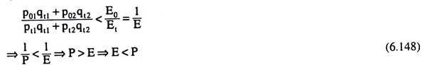
Therefore, (6.147) implying (6.148) gives us the condition for the consumer to be better off in the base period or, worse off in the current period.

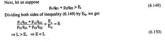
From (6.149) implying (6.150), we obtain that the cost of the base year basket at current year prices is greater than the current year expenditure. Therefore, the base year basket is not available to the consumer in the current year.

That is, he purchases the current year basket not because he prefers it to the base year basket, but because it is cheaper. Therefore, we cannot say that the consumer is better off in the current year over the base year.

Similarly, if we suppose:

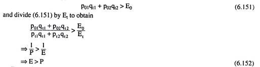
From (6.151) implying (6.152), we obtain that the cost of current year basket in the base year is greater than the base year income. Therefore, the consumer buys the base year basket in the base year not because he prefers it, but because it is cheaper than the current year basket. Therefore, here we cannot say that he is better off in the base year over the current year, or, worse off in the current year over the base year.

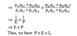
What we have obtained above is that if E > L as given by condition (6.146), the consumer is better off in the current year over the base year. On the other hand, if E < P as given by (6.148), the consumer is better off in the base year than in the current year.

We may use the indifference curves of the consumer to illustrate these points. Fig. 6.110 illustrates the first case, i.e., the consumer is better off in the current year than in the base year.

Here, in the current year, the consumer buys at the point C_t on the current year budget line and he buys in the base year at the point C₀ on the base year budget line. It is seen in Fig. 6.110 that C_t lies on the higher IC, viz., IC₂, and C₀ lies on the lower IC, viz., IC₁.

Similarly, Fig. 6.111 illustrates the second case, i.e., the consumer is better off in the base year than in the current year. It is seen in this Fig. that C₀ lying on the base year budget line, is placed on a higher IC, viz., IC₂, and C_t lying on the current year budget line, is placed on a lower IC, viz., IC₁.

From the above analysis, especially from the inequalities (6.146), (6.148), (6.150) and (6.152), we may distinguish between four cases:

(i) E is greater than both L and P (E > L, E > P). Here by (6.146), i.e., E > L, the consumer is better off in the current year over the base year. On the other hand, by (6.152), i.e., E > P, the standard of living does not fall in the current year. Hence, the individual is definitely better off in the current period.

(ii) E is less than both P and L (E < P, E < L). Here it follows from (6.148) that if E < P, the consumer would be better off in the base year, and it follows from (6.150) that if E < L, the consumer would not be better off in the current period. Again, we obtain an unequivocal answer that if E < P and E < L, then the consumer would be better off in the base period, i.e., his standard of living falls in the current period from what it was in the base period.

(iii) L > E > P. If L > E, or, E < L, then by (6.150), it cannot be said whether the consumer would be better off or worse off in the current period over the base period, and if E > P, then by (6.152), we cannot say that he would be better off in the base year. Consequently, in this case, no definite conclusion can be drawn in respect of improvement or deterioration in the standard of living of the consumer between the two periods.

(iv) P > E > L. If P> E, or, E < P, then by (6.148) the consumer’s standard of living falls in the current period, since he prefers the base year bas­ket to the current year one, and if E > L, then by (6.146), the consumer’s standard of living increases in the current year, since he prefers the current year basket to that of the base year.

Therefore, in this case also we cannot draw any definite conclusion regard­ing a change in the consumer’s welfare, and this is the situation where the weak axiom of the revealed pref­erence theory has been violated.

This situation is illustrated in Fig. 6.112. Here the base period budget line is P₀P’₀ and the current period budget line is P₁P’₁. Let us suppose that the consumer chose R (q₀₁, q₀₂) on IC₁ when the budget line was P₀P₀‘and T (q_t1, q_t2) on IC₂ when the budget line was P₁P₁‘. Since LL’ lies below P₁P₁‘ and is parallel to it and since R is on LL’ and T is on P₁P₁‘, it must be true that expenditure at R at (p_t1, p_t2) must be less than that at T at (p_t1, p_t2), i.e., we would have

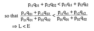
Also, since the point T (q_t1, q_t2) is on MM’ which is parallel to p₀p₀ but lies below it, T has the same prices as p₀p₀’ but has less expenditure than the point R (q₀₁, q₀₂) which lies on P₀P₀’, i.e., we have

Thus, we have P > E > L. But in this case, there is inconsistency. This is also obvious from Fig. 6.112. The consumer could have purchased T in the base period, since T lies below the base period budget line p₀p₀’, but he actually chose R, implying that he prefers R to T.

But in the current period, he could have had R, since R lies below the current period budget line P₁P₁‘, but he chose T, implying that he prefers T to R.

This is inconsistent if his tastes remain unchanged between the base period and the current period, and the weak axiom of revealed preference is not complied with. This inconsistency is also reflected in the fact that the ICs through R and T, viz., IC₁ and IC₂, have not been obtained to be non-intersecting—they have intersected at the point S.

We have seen, therefore, that it is sometimes possible to determine whether the consumer’s standard of living has increased or decreased by means of index number comparisons. However, there may be situations where we cannot arrive at any definite conclusions or where the results may be contradictory.

Example 1:

When two commodity baskets are purchased by the consumer at two different points in time, explain how price weighted quantity indices may be used to verify the weak axiom of revealed preference.

Solution:

We have to explain how price-weighted quantity indices may be used to verify the weak axiom of revealed preference. Let us suppose that in the base period ‘0’, a consumer is observed to purchase the combination q₀ (q₀₁, q₀₂) of two goods Q₁ and Q₂ at the price set p₀ (p₀₁, p₀₂) and in the current period ‘t’ he is observed to purchase the combination q_t (q_t1, q_t2) of the goods at the price set p_t (p_t1 , p_t2).

Therefore, the costs of purchasing the combination q₀ at the price set p₀ and p_t are

Again, the costs of purchasing the combination q_t at the price set p₀ and p_t are

In the base period, the consumer purchases the quantity set q₀ at the price set p₀. If he happens to prefer q₀ to q_t, then by definition, the cost of the quantity set q₀₂ must be less than, or, (at most) equal to that of purchasing q₀ at p₀, i.e.,

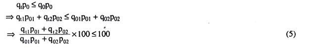
Since the left-hand side of (5) is, by definition, the Laspeyre’s base year price weighted quantity index (L), we obtain the condition for q₀ at p₀ to be preferred by the consumer to q₀ at p₀ as

L ≤100 (6)

Again, in the current period, the consumer is observed to purchase the combination q_t at price p_t. However, if the weak axiom of revealed preference is to be satisfied then he must not prefer q_t at p_t to q₀ at p_t. Therefore, we may conclude that he purchases q in the current period because it is cheaper than q₀, i.e.,

Since the left-hand side of (7) is by definition the Paasche’s current year price weighted quantity index (P), we obtain the condition for p_t at q_t to be cheaper than p₀ at q_t as

P < 100                              (8)

(6) and (8) give us that the weak axiom of revealed preference would be satisfied if the Laspeyre’s and Passche’s quantity indices both are less than 100. Of course, L may be at most 100. Here 100 is the base period index numbers for both the formulas.

Example 2:

A consumer is observed to purchase x₁ = 20, x₂ = 10 at the prices p₁ = 2 and p₂ = 6. He is also observed to purchase x₁ = 18 and x₂ = 4 at the prices p₁ = 3 and p₂ = 5. Is his behaviour consistent with the weak axiom of revealed preference?

Solution:

From the given data, we obtain:

(i) The cost of the combination (x₁= 20, x₂ = 10) at the prices (p₁ = 2, p₂ = 6) is

E₁ = 20×2 + 10×6 = 100

(ii) The cost of (x₁ = 18, x₂ = 4) at the prices (p₁ = 2, p₂ = 6) is

E₂= 18×2 + 4×6 = 60

(iii) The cost of (x₁ = 18, x₂ = 4) at the prices (p₁ = 3, p₂ = 5) is

E₃ = 18×3 + 4×5 = 74

(iv) The cost of (x, = 20, x₂ = 10) at the prices (p₁ = 3, p₂ = 5) is

E₄ = 20×3 + 10×5= 110

From above, it is obtained that the consumer buys the first set of goods, (20, 10), not because it is cheaper than the second set but because he prefers it to the second set, since the cost of the former, E₁ = 100, is greater than the cost of the latter, i.e., E₂ = 60.

However, when he purchases the second set, not the first one, at the prices (p₁ = 3, p₂ = 5), he does this because it is cheaper than the first set, not because he prefers this set to the first set, since the cost of the second set, i.e., E₃ = 74, is less than that of the first set, i.e., E₄ = 110.

Therefore, the consumer’s behaviour is consistent with the weak axiom of revealed preference.

Convexity and Concavity:

Convex and Concave Functions:

Let us refer to Fig. 6.113. A function f (x) represented by the curve ABCDE, is convex over the interval (a, b) if we have

In Fig. 6.113, point S has divided the line segment BD in the ratio 1 – λ: λ. Therefore, the x and y coordinates of point S are

OT = λx₁, +(1 -λ)x₂

and ST = λf(x₁) + (1 -λ)f(x₂)

The function f(x) is said to be strictly convex over the interval (a, b) if strict inequality holds in (6.153) for all 0 < λ < 1.

Let us again refer to Fig. 6.113. A function f(x), now represented by the curve FBGDH is concave over the interval (a, b) if we have

f [λx₁ + (1 -λ)x₂] ≥ λf(x₁) + (1 – λ)f(x₂)                    (6.154)

and the function is strictly concave if strict inequality holds in (6.154) for 0 < λ < 1.

Quasi-convex and Quasi-Concave Functions:

By definition, a function f(x) is quasi-convex over the interval (a, b) if we have

f [λx₁ + (1 -λ)x₂] ≤ max [f(x₁), f(x₂)]                        (6.155)

for all x₁ and x₂ in the interval and all 0 ≤ λ ≤ 1. The function f(x) is strictly quasi-convex if strict inequality holds in (6.155) for 0 < λ < 1.

In Fig. 6.114, the curve A’BC’DE’ represents, by definition, a quasi-convex function over the interval (a, b).

Let us now come to quasi-concavity. A function f(x) is quasi-concave over an interval (a, b) if we have

f[λx₁ + (1 – ₁)x₂] ≥ min [f(x₁), f(x₂)]                               (6.156)

for all x₁ and x₂ in the interval (a, b) and for all 0 ≤ λ ≤ 1. The function is strictly quasi-concave if strict inequality holds in (6.156) for 0 < λ < 1. In Fig. 6.114, the curve F’BG’DH’ represents, by definition, a quasi-concave function over the interval (a, b).

At the end of our discussion of convex and concave curves, let us note that, as per the definitions, a convex function is also quasi-convex for the former also satisfies (6.155), but a quasi-convex function cannot be a convex function for it does not satisfy (6.153). Similarly, a concave function is also quasi-concave for it satisfies also (6.156), but a quasi-concave function cannot be concave for it does not satisfy (6.154).

Geometrical Illustrations:

From our discussions above we obtain the following with illustrations in Fig. 6.113:

(i) The curve, ABCDE, representing a function, f (x), is convex over a certain interval (a, b) if the line segment, BD, joining any two points, B and D, on the function in the said interval lies on or above the curve; and if the line segment lies throughout above the curve, it is said that the function is strictly convex.

(ii) On the other hand, a function f(x), viz., FGDH, is concave over a certain interval (a, b) if the line segment joining any two points, B and D, on the function in the said interval lies on or below the curve; and if the line segment lies throughout below the curve, it is said that the function is strictly concave.

We also obtain the following with illustrations in Fig. 6.114.

(iii) A function f(x), viz., A’BC’DE’, is quasi-convex over a certain range between x = a and x = b, if at any x = h in the range, we have f(h) ≤ max [f(a), f(b)], and if the strict inequality holds, the function is said to be strictly quasi-convex.

It may be noted that a convex function is also quasi-convex, but a quasi-convex function cannot be convex, for some quasi-convex functions, like A’BC’DE’, may lie above the line segment joining the points on the function at x = x₁ and x = x₂, which a convex function cannot.

(iv) Lastly, a function f(x), like F’BG’DH’, is quasi-concave over a certain range between x = x₁ and x = x₂, if at any x = h in the range, we have f(h) ≥ min [f(x₁), f(x₂)]; and if the strict inequality holds, the function is said to be strictly quasi-concave. It may be noted here that a concave function is also quasi-concave.

But a quasi-concave function cannot be concave, for some quasi-concave functions, like F’BG’DH’, may lie below the line segment joining the points on the function at x = x₁ and x = x₂, which a concave function cannot.

Utility Function for Strictly Convex Indifference Curves:

Our question here is what types of utility function will produce strictly convex indifference curves (ICs) and thus satisfy the second-order condition. Two functions that may be accepted as such utility functions have been shown in Fig. 6.115. Part (a) of the Fig. 6.115 gives us a smooth strictly concave function.

Because of the assumption of positive marginal utilities, we have only shown the ascending portion of the dome-shaped surface. When this surface is cut with a plane parallel to the xy-plane, we obtain for each such cut a curve which will become a strictly convex downward sloping IC with respect to the xy-plane.

Strict concavity in a smooth utility function is, therefore, sufficient to fulfill the second-order condition (SOC) for utility-maximisation. However, if we examine part (b) of Fig. 6.115, it would be evident that strict concavity is not necessary for the SOC. This is because the strictly convex ICs can also be obtained from the utility function given in part (b) of the figure, which is not strictly concave—in fact, not even concave.

The function in Fig. 6.115 is generally shaped like a bell. Of course, we have shown here only the ascending portion of the bell. The surface of this function is called strictly quasi-concave.

The geometric property of this function is that, for any pair of distinct points u and v in its domain, if the line segment uv (which is assumed to lie entirely in the domain) gives rise to the arc MN on the surface, and if M is lower than or equal in height to N, then all the points on arc MN other than M and N must be higher than M.

[Algebraically, a function f is said to be strictly quasi-concave if, for any two distinct points in its domain like u and v, and for all values of λ, 0 < λ < 1, we would have:

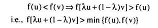
The quasi-concavity of the function in Fig. 6.115 may be verified by examining such arcs as MN (N higher than M) and M’N’ (M’ and N’ being of equal height). We have to note here that in the case of arc M’N’, it is the dotted arch that lies directly above the line segment u V, not the solid curve, which possesses the property of a quasi-concave function.

The interesting thing, however, is that the strictly concave function in Fig. 6.115(a) is also strictly quasi-concave.

From what we have obtained, we may conclude that only a smooth, increasing, strictly quasi-concave utility function would generate strictly convex ICs. Such a function may have convex as well as concave portions, as shown in Fig. 6.115(b) so that the marginal utilities may be either increasing or diminishing.

From this it follows that strict convexity of ICs does not imply diminishing MUs. However, if we accept the stronger assumption of a strictly concave utility function, then we may have the features of both diminishing MU and strictly convex ICs at the same time.