2 Main Reasons for the Change in Equilibrium | Consumer Behaviour

The equilibrium of a consumer is explained when the following two conditions are fulfilled.

These are:

(i) The slope of the indifference curve is equal to the slope of the budget line

(ii) The indifference curve is convex to the origin

Further, in developing the equilibrium condition, we assume that the money income and the prices of the two goods that a consumer purchases remain fixed. Now, if one of these variables (such as money income, price of one good) change the equilibrium of a consumer would also undergo a change.

Here we will examine the impact of a change in money income on the demand for both the goods X and Y, while the prices of both X and Y remain constant. This is illustrated in Figs. 2.29-2.33.

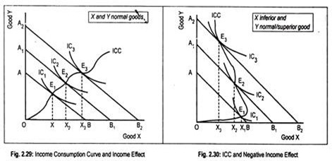
An increase in money income, holding all prices constant, leads to a parallel outward shift in the budget line. In Fig. 2.29, AB is the initial budget line and the initial equilibrium point is E₁ on IC₁ where the consumer consumes OX₁ of X and E₁X₁ of Y. As money income rises, the budget line AB shifts to the right in a parallel manner.

This new price line A₁B₁ is tangential to the indifference curve IC₂ at point E₂. Corresponding to this equilibrium point E₂, the consumer buys more of X and more of Y. By the same logic, E₃ is another equilibrium point where the budget line is A₂B₂. This new equilibrium point or optimal consumption bundle suggests larger consumption of both X and Y.

By joining all the tangency points or the equilibrium points we get a curve known as income consumption curve (ICC) or income expansion path (IEP) since this curve depicts the relationship between changes in the consumer’s income and his demand.

The locus of successive equilibrium points is called the income consumption curve which shows the quantities of X and Y demanded at different income levels. This income consumption curve traces out ‘income effect’ which shows the reaction of the consumer to income changes. Income effect may be positive or negative.

In Fig. 2.29, income effect is positive since the consumer purchases more of both X and Y when money income rises. Thus, goods X and Y are normal or superior goods. A normal good is one whose income effect is positive. As income consumption curve is upward sloping, income effect is positive for both the goods— X and Y.

However, there is no guarantee that a consumer will always behave in the manner as described in Fig 2.29. It may happen that a consumer might purchase less of a commodity even if his money income rises. This is shown in Fig. 2.30 where the income consumption curve is backward bending.

This means that, as money income rises, the consumer purchases less of X but more and more of Y. Thus, for good X, income effect is negative and, for good Y, it is positive. Thus, good X is an inferior good. An inferior good is one for which income effect is negative. However, since income effect for good Y is positive, good Y is called normal or superior good.

Truly speaking, good Y may be called an ultra-superior good. Thus, it is clear that the two goods cannot be inferior at the same time— if one good becomes inferior the other must be normal or superior. However, the two goods can be normal or superior at the same time.

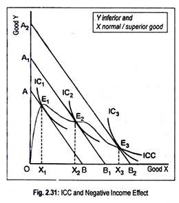
In Fig. 2.31 we have drawn a forward- falling ICC. This figure suggests that, as income rises, demand for Y decreases while that of X rises.

Thus, income effect of good Y is negative and that for good X is positive. In other words, good Y becomes inferior while good X becomes normal or superior good. Or following our definition, good X can be labeled as an ultra-superior good. So, the two goods cannot be inferior at the same time.

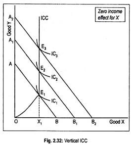
In Fig. 2.32 income consumption curve becomes parallel to the vertical axis. This means that, as income rises, consumption of Y rises while consumption of X remains stationary at OX₁. Thus, income effect for good Y is positive but for good X it is zero.

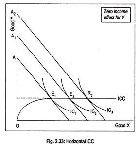
Similarly, in Fig. 2.33, we have an income consumption curve parallel to the horizontal axis. It suggests that, for good Y, income effect is nil while that for good X it is positive.