Theoretical Foundations Demand of Consumer Behaviour

The below mentioned article provides an overview on Theoretical Foundations Demand of Consumer Behaviour.

Analysis of Consumer behaviour:

In the analysis we did not proceed further to derive the demand curves or develop their characteristics. Since mar­ket demand is directly related to the way consu­mers are willing and able to act, it is necessary to study consumer behaviours in order to build the the­oretical foundations of demand.

It is absolutely es­sential for marketing managers to be aware of what underlies demand in order to understand, estimate, and forecast the demand for the products they sell. We propose to demonstrate how the demand curve of an individual consumer is derived. We shall also examine the determinants of this demand function.  

The basic theory of consumer behaviour is sim­ple enough. It starts from the proposition that most people do not have incomes sufficient to buy as much as they desire of every good or service.

In­stead, the consumer attempts to attain the most preferred level of consumption — combination of goods and services — with a fixed level of money income and a fixed set of commodity prices. Thus an analysis of consumer behaviour is basically a study of the problem of constrained optimization.

The Utility Function:

A rational consumer seeks to maximize his level of satisfaction or utility. The word utility refers to the want-satisfying capacity of a commodity. More precisely, the consumer chooses the goods and ser­vices that maximize utility (subject to a budget con­straint).

Utility is simply defined as follows:

Definition:

Utility is an individual’s perception of his own satisfaction from consuming any specific combination of goods and services.

The utility function of a representative consu­mer is expressed in the form:

U = ƒ (X₁, X₂, X₃ …….. X_n)

where X_i is the amount of the i-th good or ser­vice to be consumed. Here U stands for total utility or the sum-total of satisfaction obtained by consum­ing a number of commodities. The value of U, which is some index of utility, depends upon the quanti­ties of n number of goods consumed.

For the sake of simplicity we may assume that the consumer consumes only two goods (or services)- X and Y, and he has to choose among bundles con­sisting of only X and Y.

So the utility function can be expressed as:

U = ƒ (X, Y)

where X and Y denote respectively the levels of consumption of the two commodities.

The theory of consumer behaviour is based on a number of simplifying assumptions. The following two assumptions are most important.

Complete Information:

Firstly, the consumer is supposed to have com­plete information regarding his consumption deci­sions. He is aware of the full range of goods and services available and the capacity of each to pro­vide satisfaction (or utility). Furthermore he knows the exact market price of each goods. He also knows his income during the time period under consideration.

Preference Ordering:

The second fundamental assumption is that the consumer is able to rank all conceivable combina­tions of commodities on the basis of the ability of each combination to provide satisfaction or utility. When faced with two or more combinations or bundles of goods, the consumer can determine his or­der of preference among them.

This point may be explained with an example. Let up suppose a consumer is confronted with the bundles consisting of different combinations of two goods. Bundle 1 consists of Amul chocolates and one soft drink (say, Limca). Bundle 2 consists of three soft drinks.

Ranking the two bundles, the consumer can make one of three possible responses:

(1) He may prefer bundle 1 to bundle 2.

(2) He may prefer bundle 2 to bundle 1.

(3) He may be equally satis­fied with (indifferent between) either.

The same argument holds when ranking any two bundles of goods and services. The consumer either prefers one bundle to the other or is indifferent be­tween the two. A consumer who is indifferent be­tween two bundles clearly feels that either bundle would yield the same level of satisfaction or utili­ty. A preferred bundle would yield more utility than the less-preferred bundle.

Relations:

Consumers are assumed have a prefer­ence pattern that:

(1) Establishes a rank ordering of all bundles of goods and

(2) Compares all pairs of bundles, indicating that bundle 1 is preferred to bundle 2,2 is preferred to 1, or the consumer is indif­ferent between 1 and 2.

In a three (or more) way comparison, if 1 is preferred (indifferent) to 2, and 2 is preferred (indifferent) to 3, 1 must be preferred (indifferent) to 3. This is known as the transitivity assumption. A large bundle, in the sense of having at least as much of each good and more of another, is always preferred to a smaller one. More is pre­ferred to less. This is known as the relationality assumption.

Indifference Curves:

A fundamental tool for the analysis of consumer behaviour is an indifference curve.

It is defined as follows:

Definition:

An indifference curve is a locus of points, showing alternative combinations or bundles of goods and services, each of which yields the same level of total utility or satisfaction to the consumer. Indifference curve analysis is based on the as­sumption that the consumer chooses among bundles consisting of only two goods. This assumption makes possible diagrammatic analysis of consumer behavi­our.

Figure 9.1 shows a typical indifference curve with the normal downward slope. The quantity of some goods X is plotted along the horizontal axis; the quantity of goods Y (say, all other goods) is plotted along the vertical axis.

All the alternative combinations of goods X and Y along indifference curve I are supposed to yield the consumer the same level of satisfaction or utili­ty. Differently put, the consumer is indifferent among all points such as A, with 10 units of X and 50 units of Y; point B, with 20X and 35Y, point C, with 40X and 18Y; and so on.

At any point on Curve I, we can take away some amount of X and add some amount of Y (though not necessarily the same amount) and enable the consumer to enjoy the same level of utility. By contrast may we add X and take away just enough Y so that he continues to enjoy the same level of satisfaction or utility. In this case the consumer will be indifferent between the two combinations.

The indifference curve is negatively sloped. The implication is that the consumer derives utility from both goods. Thus, if we add X, we must take away Y in order to keep the level of utility un­changed. If the curve in Figure 9.1 would start slop­ing upward at, say, 70 units of X, it would mean that the consumer has so much X that any addi­tional X would reduce utility.

In such a situation to keep the consumer at the same level of utility when X is added, more Y must be given to compen­sate for lost utility from having X. In a like man­ner, if the curve begins to bend backward at, say, 70 units of Y, it would imply that the consumer experiences fall in utility with increases in Y.

Since utili­ty is a subjective concept and cannot be measured in terms of numbers, we generally do not assume that a specific number measuring utility is assigned to an indifference curve.

We can also speak about the shape of the indif­ference curve. An indifference curve is convex to the origin. The implication is that as the consumption of X is increased relative to Y, the consumer is will­ing to accept a smaller reduction in Y, for an equal increase in X, in order to stay on the same indiffer­ence curve and enjoy the same level of utility or satisfaction. This property is also illustrated in Figure 9.1.

Suppose we begin at point A with 10 units of X and 50 units of Y. In order to increase consumption of X by 10 units, to 20, the consumer is willing to reduce consumption of Y by 15 units, to 35. On the indiffer­ence curve I, the consumer will be indifferent be­tween the two combinations A and B. Next we may begin at C, with 40Xand 18Y.

Beyond this stage, to gain an additional 10 units of X (a move to point D), the consumer is willing to give up only 6 units of Y, much less than the 15 units willingly given up at A. The indifference curve is convex to the origin be­cause of diminishing marginal rate of substitution. This concept may be explained now.

The Marginal Rate of Substitution:

The slope of an indifference curve measures the marginal rate of substitution.

This is defined as fol­lows:

Definition:

The marginal rate of substitution of X for Y measures the number of units of Y that must be sacrificed per unit of X added, so as to yield the same level of utility. In fact, the indifference curve approach is based on the law of substitution.

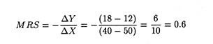
In Figure 9.1, it is clear that the consumer is in­different between combination A (10X and 50Y) and b (20Y and 35Y). Therefore, the rate at which the consumer is willing to substitute X and Y is

The marginal rate of substitution is 1.5 which im­plies that the consumer is willing to sacrifice 1.5 units of Y for each additional unit of X.

The margi­nal rate of substitution is expressed as:

If the consumer moves from C to D along I, the MRS is

In this case the consumer is willing to forego only 0.6 units of Y to acquire an additional unit of X. The marginal rate of substitution is thus given by the negative of the slope of an indifference curve at a point. It is defined only for movements along a giv­en curve. It is also known as the marginal signifi­cance.

It is clear that the MRS diminishes along an in­difference curve. When a consumer is having a small amount of X relative to Y, he is ready to sac­rifice a large amount of Y to gain another unit of X. When he is having less Y relative to X, he is will­ing to give us less Y in order to gain another unit of X.

Thus the negative of the slope of the tangent R at point A is the MRS of X for Y at the point. The same is true for tangent T at point C. These tangents indicate that the slope of the indifference curve, and hence the MRS declines as X is increased rela­tive to Y.

An Indifference Map:

A consumer need not have only one indifference curve. Since the indifference curve shows an imag­inary situation he can have many such curves. All such curves together constitute the indifference map of the consumer.

An indifference map is simply a collection or a set of two or more indifference curves. Figure 9.2 shows a typical indifference map, made up of four indifference curves, I, II, III and IV.

An indifference curve which lies above and to the right of another represents a higher level of utility and thus a preferred combination of the two commodities. Thus any combination of X and Y on IV (line A'”) is pre­ferred to any combination on III (A”), any combina­tion on III (such as A”) is preferred to any on II (A’), and so on.

Thus, any point on a higher indifference curve is better than any point on a lower indiffer­ence curve. In short, all combinations of X and Y on the same indifference curve are equally valued by the consumer; all combinations lying on a higher curve are preferred.

A property of indifference curves is that they cannot meet or intersect. If they do, the consumer will be behaving inconsistently. Here it suffices to note that the X-Y space in an indifference map may contain an infinite number of indifference curves. Since each point in the space lies on one and only one indifference curve, indifference curves can­not intersect.

The Marginal Utility Approach:

The concept of marginal utility can provide fur­ther insight into the properties of indifference curves. In economics the word ‘margin’ always re­fers to anything extra.

We define marginal utility as follows:

Definition:

Marginal utility is the addition to to­tal utility obtained by consuming one extra of one unit of a commodity to the current rate of consump­tion, holding constant the amounts of all other goods consumed.

Although utility is not measurable either in terms of money or in terms of numbers, we can relate marginal utility to the marginal rate of substitu­tion along an indifference curve. Let us assume that total utility (U) depends upon the level of con­sumption of only two goods, X and Y. The total change in utility following a small change in both X and Y can be represented as

∆U = [(MU of X) x ∆X]+[(MU of Y) x ∆Y]

All combination of goods indicated by the dif­ferent points on the same indifference curve yield the same level of utility. Thus, ∆ U is zero for all changes in X and Y that would keep the consumer on the same indifference curve. Thus, if ∆U = 0 if fol­lows that

where (-∆Y/∆X) is the negative of the slope of the indifference curve, or the MRS. The MRS is also known as the desired rate of commodity substitu­tion.

The Consumer’s Budget Constraint:

Indifference curves are derived from the prefer­ence pattern of the consumers and show the desire of the consumer. But the desire to buy a commodity is not enough. The consumer must have sufficient capacity to do so. His capacity depends on his bud­getary (income) position.

Since the consumer is sup­posed to have fixed income at a particular point of time he has to operate under budget constraint. A consumer reaches equilibrium and maximizes utili­ty when his desire coincides with his capacity.

The demand functions indicate what consumers are both willing and able to buy. Consumers are constrained in what they are able to buy by a fixed level of money in­come and fixed set of (market-determined) prices. We now turn to an analysis of the constraint that the consumer faces, i.e., the budget or income con­straint.

The Budget Line:

A consumer having limited income has to spend it in such a way that gives the maximum possible satisfaction. Suppose fixed money income is denot­ed as M. This is the maximum amount that can be spent on the two goods, X and Y. Thus, the expendi­ture on X (P_x. X) plus the expenditure on Y (P_y.Y) must equal income (M):

M = p_xX + p_yY

This equation can be rewritten as:

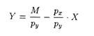
This is the equation of the budget line which can be defined as follows:

Definition:

A budget line is the locus of points showing all combinations or bundles of the two goods (i.e., X and Y) that can be purchased by spending the entire money income of the consumer.

The first term, M/P_y on the right hand side shows the amount of Y the consumer can buy if he spends all his income on Y. This is the intercept of the budget line. Suppose his income is Rs. 1,000 and the price of Y is Rs. 5 per unit. If the consumer spends all his income on Y, he can buy 200 units of Y.

If the consumer spends all his income on X, he can buy M/p_x units of X. This is shown by the horizontal distance OA. Thus, the slope of the budget line is BO/OA = M/p_y + M/p_x = M/p_y . p_x/M = p_x/p_y. Since some units of Y have to be sacrificed to get more of X, this price ratio p_x/p_y is always negative.

This ratio is also known as the actual rate of commodity substitution in the sense that it indicates the rate at which Y can be substituted by X or X can be substi­tuted by Y in the market place (where actual trans­actions occur). Since the slope of the budget line shows price ratio (or relative price of X in terms of Y), it is also known as the price line.

The slope of the line (-p_x/p_y) indicate the amount of Y that must be foregone if one more unit of X is to be obtained from the market place. Suppose the price of Y is Rs. 5, and the price of X is Rs. 10. For every additional unit of X, the consumer has to sac­rifice Rs. 10 worth of Y, or two units of Y.

Thus, the rate at which a consumer can exchange Y for more X is 10/5 = 2; two units of Y for one of X. If, instead, the price of X is Rs. 2.50, the rate that Y can be traded for X is 2.50/5.00 = 1/2. For every additional unit of X, the consumer must give up 1 /2 unit of Y.

A hypothetical budget line is shown in Figure 9.3. The line BA shows all possible combinations of Y and X that can be purchased with a fixed amount of money income and a fixed set of commodity pric­es.

Shifting the Budget Line:

If money income (M) or the price ratio (p_x/p_y) change, the budget line will look different. Panel A of figure 9.4 shows the effect of changes in in­come. Let us begin with the original budget line BA.

Now suppose money income increases but the prices of X and Y remain constant. Since there is no change in the prices, the slope of the budget line remains unchanged. But since money income increases, M/p_y, the vertical intercept must increase (shift up­ward).

Thus, if the consumer spends all his income on good Y, he will be able to buy more units than he could afford earlier. An increase in income lead to a parallel right hand shift of the budget line from BA to RN. The increase in income enables the consu­mer to acquire the set or combinations of goods that he previously desired but could not afford.

Alternatively, we may start with budget line BA and allow money income to fall. In this case the set of possible combinations of goods that can be ac­quired from the market falls. The vertical inter­cept decreases, causing a parallel leftward shift of the budget line to FZ.

Panel B shows effect of changes in the market price of one of the purchasable goods—say good X. Let us start once gain with the budget line BA, then let the price of X fall. Since M/p_y does not changes, the vertical intercept remains unchanged at B. But when p_x declines, the budget line becomes flatter and the absolute value of the slope, p_x/p_y falls.

In Panel B the budget line rotates clockwise from BA to BD. In other words, if the price of X falls, more X can be purchased with the same amount of money if the en­tire money income is spent on X. Thus in Figure 9.4(b) the horizontal intercept increases from OA to OD.

An increase in the price of goods X produces exactly opposite effects — it causes the budget line to rotate anti-clockwise from BA to BC and thus be­came steeper. That is, if p_x increases, the absolute value of the slope of the line, p_x/p_y, has to increase. The budget line becomes steeper, while the vertical intercept remains unchanged.

Thus, the basic point to note is that an increase (decrease) in money income causes parallel out­ward (backward) shift of the budget line. By con­trast, an increase (decrease) in the price of X causes the budget line to pivot backward (outward) around the original vertical intercept.

Utility Maximization and Consumer Equilibrium:

Thus we have developed two important tools of our analysis of the theory of consumer demand. The indifferent curve shows what the consumer is willing to buy while the budget line indicates what he is capable of buying with a fixed level of money income and a fixed set of commodity prices.

The consumer reaches equilibrium and thus maxi­mizes utility when his desire coincides with his capacity, or the desired rate of commodity substi­tution (i.e., MRS) is equal to the actual rate of com­modity substitution (i.e., the price ratio).

A rational consumer, whose objective is to reach the point of maximum satisfaction or welfare, will always try to reach the highest possible indiffer­ence curve permitted by the budget line. We may now examine how the optimization goal of the con­sumer is accomplished.

Maximizing Utility Subject to the Budget Constraint:

In Figure 9.5 we put the budget line (of Fig. 9.3) and the indifference map (of Fig. 9.2) together. With this budget line the consumer is capable of reaching indifference curve III.

Indifference curve IV is beyond his reach because of limited income (or fixed budget). Clearly the highest level of satis­faction possible is attained at P on indifference curve III, where the individual consumes X* units of X and Y* units of Y, respectively.

Other bundles such as Z or S are attainable but lie on lower indifference curve and are therefore less preferred. If he chooses Z or S one of the major properties of indifference curves will be violated (i.e., an indifference curve which lies above and to the right of another shows a preferred combination of the two commodities).

Thus it logically follows that any point on a higher indifference curve is bet­ter than any point on a lower indifference curve. Let us consider the bundle given by point R.

The consu­mer could move upward along the budget line, sacri­ficing X and acquiring extra Y, through combination such as that at S. The consumer would stop substi­tuting Y for X only when P is reached, because through such substitution he will be able to reach a higher indifference curve.

The consumer would surely not move beyond point P to points such as Z, because that would take him to a lower indifference curve. If the consumer started at combination Z, for example, he could sub­stitute X for Y along the budget line and attain higher and higher levels of utility until P is reached.

Thus the consumer reaches equilibrium and max­imizes utility by choosing the combination at which the marginal rate of substitution (the slope of the indifference curve) or the desired rate of commodity substitution equals the price ratio (the slope of the budget line) or the actual rate of com­modity substitution.

Thus consumer reaches equilibrium at the point at which his desire is the same as his capacity.

To explain the logic of equilibrium further we may proceed a step ahead. To prove that P is the only equilibrium point in Fig. 9.5 we have to dis­prove that no other point such as Z and S can be a point of equilibrium. Let us consider a combination such as S in Figure 9.5. At this point, the marginal rate of substitution is less than the price ratio.

Let us suppose at this points MRS = 2 and P_x/P_y = 4. The consumer is willing to sacrifice one unit of X to obtain extra two units of Y. The price ratio per­mits him to obtain four units of Y for each unit of X sacrificed. Thus the consumer will be better off if he substitutes X for Y.

Conversely, we let us suppose the consumer is at a point such as Z, where the MRS exceeds the price ratio. Suppose at this point the MRS is six and the price ratio remains four. The consumer is willing to forego six units of Y to get one additional unit of X. The price ratio allows the consumer to forego only four units of Y to obtain each additional unit of X. Thus the consumer will be better off if he substi­tutes Y for X.

Thus one of the fundamental propositions of the theory of consumer demand is that the maximiza­tion of satisfaction subject to a limited money in­come occurs at the combination of goods for which the MRS of X for Y equals their price ratio.

Marginal Utility Interpretation:

We have defined the MRS at the ratio of the two marginal utilities — MU_X and MU_y. Thus equi­librium occurs when

 

 

 

 

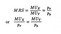
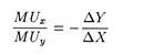
This implication of his condition is that the mar­ginal utility per rupee spent on goods X equals the marginal utility per rupee spent on Y. This princi­ple certainly looks plausible. To see why this con­dition should hold let us suppose that the condition did not hold and that

The marginal utility per rupee spent on good X is less than the marginal utility per rupee spent on Y. The consumer can take rupees away from X and spend them on Y.

As long as the inequality holds, the lost utility from each rupee taken away from X is less than the added utility from each extra rupee spent on Y, and the consumer go on substituting for X. As the consumption of X falls the marginal utility of X will rise. Contrarily as Y increases, its margi­nal utility falls. The consumer go on substituting un­til MU_x/p_x equals MU_x/p_y.

Alternatively if

the marginal utility per rupee spent on X exceeds the marginal utility per rupee spent on Y. The con­sumer takes rupees away from Y and buys addition­al X, continuing to substitute until the equality is reached. To obtain the highest possible satisfaction from a limited money income, a consumer so allocates his money income that the marginal utility per rupee spent on each good is the same for all commodities purchased.

Deriving Demand Curves:

Demand is the quantities of a good the consumer is willing and able to purchase at each price holding other things constant (i.e., the ceteris paribus assump­tion).

We have just noted that a consumer maximiz­es utility when the desired rate of commodity sub­stitution is equal to the actual rate of commodity substitution. Now we shall see that the two theo­ries are inter related in the sense that the theory of demand can be easily derived from the theory of consumer behaviour.

In Figure 9.6 we show this relation. We also show how the demand curve of our representative consumer is actually derived from his indifference map. In the top half of the diagram we show the consumer’s reaction to the change in the market price of one of the purchasable commodities (X) and his successive equilibrium points. We begin with a fixed level of money income and fixed prices of the two goods.

The corresponding budget line is given by budget line in Figure 9.6. Let the original price of X be p₁ the consumer maximizes utility where budget line is tangent to indifference curve I, as at point F where he consumers X₁ units of X. Clearly, p₁, x₁ is one point (shown by F’) on this consumer’s demand curve for X.

Now, following the definition of demand we hold money income and the price of the other good constant, while allowing the price of X to fall from p₁ to p₂. The new budget line is now Bud­get Line 2. Since money income and the price of Y remain constant, the vertical intercept remains un­changed, but since the price of X has fallen, the budget line becomes flatter along the X axis.

With this new budget line, the consumer now maximizes utility where budget line 2 is tangent to indiffer­ence curve II at point F, consuming x₂ units of X. This, p₂, x₂ must be another point (shown by F) on the de­mand schedule.

Next, allowing the price of X to fall further to p₃, the new budget line is 3. Again the price of Y and money income were kept unchanged. The new equilibrium is at point G on indifference curve III. At the price p₃, the consumer chooses x₃ units of X and we get another point (G’) on the consumer’s demand curve.

Thus we obtain the following demand schedule for good X.

This scheduled is graphically represented as a demand curve in price-quantity space in the bottom half of Figure 9.6. This demand curve is downward sloping because of the empirical law of demand. As we allow the price of X to fall, the quantity of X the consumer is willing and able to purchase in­creases.

Furthermore, following our definition of demand, we kept money income and the price of the other goods constant. Thus, it is clear that an indi­vidual consumer’s demand for a good is derived from a series of utility-maximizing equilibrium points. We only used three such points. But the same analysis could be extended to obtain more points on the demand curve.

In short, the demand curve of an individual con­sumer for a specific commodity relates to utility-maximizing equilibrium quantities purchased at market prices, holding constant money income and the prices of all other goods. The slope of the de­mand curve illustrates the empirical law of de­mand: the quantity demanded of the commodity varies inversely with its price.

Substitution and Income Effects:

When the price of a good falls a consumer tends to buy more of it and he substitutes that good for other goods, since the good in question has become relatively cheap (and the other good relatively expensive although nothing has happened to its absolute price).

Con­versely, when the price of a good rises, it becomes relatively expensive and the consumer tends to sub­stitute some other good for the good whose price has risen. This is called the substitution effect.

But, there is also another effect, known as the income effect. If the price of a commodity falls the consumer’s real income or purchasing power increas­es. So with the same amount of money (i.e., un­changed money income) he can buy more of the com­modity as also more of the other goods.

It is because when the price of say, X falls, a consumer can buy the same amount as before, but because of the re­duced price, he has some income left over, which can be spent on X and on the other goods Y.

Exactly the opposite thing happens when the price of goods rises. The consumer is worse off in the sense that he cannot now afford the bundle he originally chose. He is forced to consume less of the now more expensive goods, less of the other goods, or less of both. This is called the income effect. We may now analyse each effect in turn.

Substitution Effect:

The substitution effect of a change in the mar­ket price of one of the purchasable commodities is the change in the consumption of the good that re­sults when the consumer remains on the same indif­ference curve.The nature of the substitution effect is illustrated in Figure 9.7 in which we consider a fall in the price of X.

We start a situation where the consumer is in equilibrium. In Fig. 9.7 this happens at point E where the original budget line AB is tangent to in­difference curve I. The consumer chooses x₁ units of commodity X. Now suppose the price of X falls so that the budget line rotates anti-clockwise and be­comes AD.

This enables the consumer to reach a higher in­difference curve and enjoy a higher level of satis­faction or utility.

But since the substitution effect deals with changes on the same indifference curve, we may “take away” just enough of the consumer’s income so that he is neither better off nor worse off, i.e., he is permitted to stay on the same indiffer­ence curve I (as before the price fall) and enjoy the same level of satisfaction or utility.

To ensure this we may consider an imaginary situation in which we shift the budget line, AD parallelly to LZ, so that it becomes tangent to the old indifference curve I. The important point to note is that the slope of LZ reflects the new, lower price of X, but is associated with a lower money income than is the original budget line AB.

Now the new budget line LZ is tangent to the old indifference curve I at a dif­ferent point G, indicating that the consumer now chooses a larger quantity (x₂) units of X in the event of a fall in its market price.

The substitution effect is measured by the dis­tance x₁ to x₂ or the movement along I from E to G. Substitution effect is always negative-fall in price must result in an increase in demand of the good when utility is held constant. And this will al­ways be so because the indifference curve is nega­tively sloped.

That is, a fall in price causes the budget line to become flatter; so the budget line, af­ter taking away some income, must be tangent to the old indifference curve at a point with a lower slope (MRS) than was the case at the original equilibri­um. This result can be obtained only when consump­tion of the good increases.

Thus the substitution effect is the change in the consumption of a good after a change in its price, when the consumer is forced by a change in money income to consume at some point on the same indif­ference curve.

If we consider the substitution effect alone, we observe that the quantity of the commod­ity demanded must vary inversely with its price. That is, total utility held constant, ∆X/∆p_x < 0. In other words, the substitution effect explains why the demand curve for a commodity is normally downward sloping.

Thus in our analysis of substitution effect, we keep the price ratio p_x/p_y unchanged as is obvious from the fact that the two budget lines AD and LZ run parallel to each other. We allow money income (M) to change.

Income Effect:

The income effect of a price change has been de­fined by J. R. Hicks as the change in the consump­tion of a good resulting strictly from the change in real income or purchasing power. Now we keep money income (M) constant and permit the ratio (P_x/P_y) to change.

While analysing the substitution effect we not­ed that a fall in the price of a commodity makes a consumer of that goods better off in the sense of be­ing able to purchase the same combination of the two commodities and have some unspent income, i.e., the consumer can move to a higher indifference curve.

Contrarily, an increase in the price of a good makes a consumer worse off because he is unable to buy the old combination of the two goods; i.e., the consumer is now forced to move to a lower indiffer­ence curve.

Since the consumer moves to a higher or lower indifference curve, depending upon the direc­tion of the price change, and the substitution effect is measured by observing the movement of the con­sumer along the same indifference curve from one point to another, the income effect is simply the difference between the total effect of the price change — the movement from one indifference curve to another — and the substitution effect.

We can isolate these effect for a price fall in Figure 9.8. First consider Panel A. Start with bud­get line AB and equilibrium at E (x₁ units of X) on in­difference curve I. Now suppose the price of X falls and the budget line rotates to AC.

The new equili­brium is at point F on indifference curve II. The to­tal effect of the price decrease (known as the price effect) is to increase the consumption of X from x₁ to We have already noted that the movement from x₁ to x₂ (or from E to R) is the substitution effect.

Thus it logically follows that the reminder of the change x₂x₃ or the movement from R to F between indifference curves is the income effect. Thus if we return the income that was “taken away” to isolate the substitution effect, the consumer will move to a higher indifference curve II and increase his con­sumption of x further from x₂ to x₃.

In Panel A the commodity under consideration is a normal good. Con­sumption of a normal good increases when income increases but prices are constant. This is exactly what happened here when the budget line was shifted from LZ back to its original position AC.

As Figure 9.8 (Panel A) shows in the case of a normal good, the income effect reinforces the substi­tution effect. Thus, for a normal good both effects are negative. Income effect is negative because a fall in price of X and the consequent increase in real income leads to an increase in the consumption of X.

Thus when price of a normal good falls both the substitution effect and the income effect cause the consumer to purchase more of it. Likewise, when the price of the good rises, both effects will cause the consumer to purchase less of it.

We may how consider the case of an inferior good. We have noted that if a good is inferior, an increase in income, holding prices constant, causes less of the good to be consumed. Thus income effect is positive (i.e., a fall in p_x leads to a fall in the consumption of X, too);

The case of an inferior good is illustrated in Panel B of Figure 9.8. Let us start as before, with budget line AB. Equilibrium is at E on indifference curve I with x₁ being consumed. When the price X falls, the budget line becomes flatter (AC), the new equilibrium is at F on difference curve II, with x₂ be­ing consumed, the total effect is therefore shown as x₁x₃.

If we shift the new budget line back to LZ, and eliminate the income effect we prove that the sub­stitution effect is x₁x₂. Here the substitution effect outweighs the total effect; x₂ is greater than x₃ (or x₁x₂ exceeds x₁x₃). Thus for an inferior good the in­come effect partially neutralizes the substitution effect.

To test the validity of this proposition let us re­turn the income taken away when isolating the substitution effect. The budget line shift back to its original position, i.e., from LZ to AC.

Since the good is inferior, this increase in income causes less X to be consumed than was the case when the budget line was LZ. The income effect is therefore measured by the movement from x₂ back to x₃ (or the movement from R to F between indifference curves I and II).

We can see that in this case the income effect is positive — a fall in the price of X causes a decrease in the consumption of X (real income effect only). It is also possible to show that if the price of an in­ferior good rises, the income effect alone leads to an increase in consumption.

Thus if we consider the substitution effect alone, an increase (decrease) in the price of a good will cause less (more) of the good to be demanded. For a normal good, an income effect — from the consu­mer’s being made better or worse off by the price change — adds to or reinforces the substitution ef­fect so as to make price effect negative, i.e., if the price of a commodity falls, the quantity demanded of the same increases. This is known as the Slutsky theorem. The income effect in the case of an inferi­or good offsets or takes away from the substitution effect and may make the price effect positive.

Why Does the Demand Curve Slope Downward?

In the case of a normal good, it is quite obvious that price and quantity demanded are inversely re­lated. From the substitution effect alone, a fall in price leads to an increase in quantity demanded. The converse is also true.

For a normal good, the in­come effect and the substitution effect go hand in hand. Since both effects change quantity demanded in the same direction, the demand curve for a nor­mal good must always be downward sloping from left to right.

In the case of an inferior good, the income effect does not move in the same direction, and neutralise the substitution effect at least partly.

However, from Panel B of Figure 9.8, we observe that the in­come effect only partially offsets the substitution effect, so that quantity demanded still varies in­versely with price. And this is the general case: even if the commodity is inferior, the substitution effect dominates the income effect; so, the demand curve will still be negatively sloped.

It is theoretically possible that the income ef­fect for a special variety of inferior goods could out­weigh the substitution effect. In this case — the so- called Giffen goods — quantity demanded would vary directly with price and the demand curve would be upward sloping.This type of goods hard­ly exist in practice. So such goods provide an impor­tant, albeit rare, exception to the empirical Law of Demand.