Choice between Leisure and Income (With Equations)

The indifference curve theory of consumer behaviour may be applied to derive the supply curve of labour of a worker from his preference-indifference pattern between income and leisure. Income is the aggregate of expenditures on all goods and services, and so, it is a source of (positive) utility to the worker.

On the other hand, leisure is the time left with the worker after work. It is also a source of (positive) utility to the worker. The amount of income received by a worker depends upon the amount of time allocated to work.

The more is the time devoted to work, the more would be the income of the worker, and the less would be his leisure-time. Therefore, each worker faces a trade-off between consumption of goods and services represented by income and the consumption of leisure.

The Income-Leisure Space:

In Fig. 6.85, income is measured along the vertical axis and leisure on the horizontal axis. It should be noted that, since the total available time in a day is 24 hours, the sum of the leisure time and the time of work must be equal to 24 hours, assuming that the time the worker does not work is included in leisure.

In Fig. 6.85, OM on the horizontal axis measures 24 hours. Leisure is measured along the horizontal axis from O to M and work is measured from M to O. If OC hours per day is taken as leisure, then the amount of work per day is MC.

For the sake of simplicity, we shall assume here:

(i) that the individual may work as many hours per day (not exceeding 24) as he desires. The remaining part of the day he would enjoy as leisure, and

(ii) that the rate of wage per hour is a constant irrespective of the number of hours worked.

For example, if the individual works CM hours per day and receives an income of CE per day, then the rate of wage per hour is CE/CM which is equal to the numerical slope of the straight line AM.

Income-Leisure Indifference Curves:

Since both income and leisure are sources of positive utility (more-is-better) to the consumer, and the MRS between leisure and income is assumed to be diminishing, the indifference map between these two ‘goods’ for an individual would have negatively sloped and convex-to-the origin ICs.

Such an indifference map has been given in Fig. 6.86. The ICs here possess all their usual properties. The curve IQ gives us that the worker gets the same level of utility from OA of leisure (L) and OB of income (Y), and from OC of L and OD of Y, and so on.

A higher IC gives him a higher level of utility, for at any point on a higher IC, he gets more of one good at any given quantity of the other. For example, on IC₁ he gets OD of Y at OC of L, and on IC₂ he gets OE of Y (OE > OD) at the same OC of L.

The Income-Leisure Budget Line:

In Fig. 6.85, the maximum amount of leisure that the worker can enjoy per day is OM (= 24 hours). On the other hand, if he works 24 hours per day, then the maximum amount of income that he may obtain is, say, OA which is equal to the rate of wage (W) multiplied by 24.

Therefore, the straight line AM would be his budget line. The points on this line give us the income-leisure combinations that are available to him at the rate of wage OA/24= OA/OM = numerical value of the slope of the line AM. Since income diminishes as leisure increases, the slope of AM is negative.

Now, if W rises, the maximum amount of income at L = 0, would be more than OA, say, it is OB (OB > OA). Then the budget line of the worker would be BM. In other words, as W rises, his budget line would rotate clockwise about the point M.

Lastly, it may be noted here that the rate of wage itself is the price of leisure. For, to enjoy one more hour of leisure, the individual would have to work one hour less and he would have to forego one hour’s wage (i.e. W). Also, the price of income (Y) is P_Y = 1 (unit of money).

The Equilibrium Choice:

If we now superimpose the budget line AM of the worker on his indifference map as has been done in Fig. 6.87, the point of tangency E between the budget line and one of his ICs, viz., IC₂, would be his equilibrium point, for at this point he can reach the highest possible IC, i.e., highest possible level of utility, subject to his budget constraint. At the point E, he opts for the combination of OC of L and OD of Y. The point of tangency E gives us that the income- leisure equilibrium condition for the individual is

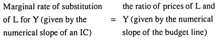
Marginal rate of substitution the ratio of prices of L and of L for Y (given by the numerical slope of an IC) = Y (given by the numerical slope of the budget line)

The Supply of Labour:

From the equilibrium analysis of an individual worker between income and leisure at any par­ticular rate of wage, we may now easily derive his supply of labour function with the help of Fig. 6.88. In Fig. 6.88 (a), at the budget line AM or at the rate of wage OA/OM = W₁ (say), and at the equilibrium point E₁ the individual’s consumption of leisure is L₁ = OL₁ and, therefore, his supply of labour is L₁* = L₁M = 24 – L₁.

Similarly, at the budget line BM or at the rate of wage OB/OM = W₂, say, (W₂> W₁), and at the equilibrium point E₂, his consumption of leisure amounts to L₂ = OL₂ (L₂ < L₁) and his supply of labour becomes L *₂ = L₂M = 24 – L₂, (L*₂ > L*₁). Here we have obtained for an individual worker, that as W rises, quantity consumed of leisure (L) diminishes and supply of labour (L*) increases.

Now, if we plot the combinations of W (which is the same as the price of leisure) and L (leisure) explicitly, in a W-L space, we obtain a curve like DD’ in Fig. 6.88 (b), which may be taken as the demand curve for leisure.

At the prices of leisure of W₁ and W₂, the individual’s demand for leisure is L₁ and L₂. In our case, as W increases, L diminishes. So, the slope of the demand curve for leisure, DD’, has been negative here.

Let us now come to the supply curve of the individual’s labour. Here, the supply of labour (hours per day) has been defined as L* = 24 – L. In part (a) of Fig. 6.88, as the rate of wage (W) increases, L diminishes and L* = 24 – L increases.

For example, at W = W₁ and W = W₂, (W₂ > W₁) we have: L* =24-L₁ =ML₁ and L*₂ = 24 – L₂ = ML₂, (L*₂ > L₁*). If we plot these wage-labour supply combinations for the individual explicitly in a W – L* space like that of part (c) of Fig. 6.88, and join these points by a curve, then that curve which is SS’ would give us the individual’s labour supply curve.

In our example, as W or the price of leisure has increased, demand for leisure has diminished, and therefore, the supply of labour has increased. That is why the supply curve of labour has been obtained to be positively sloped.

Income Effect, Substitution Effect and Price Effect of a Change in the Rate of Wage upon the Supply of Labour:

As the rate of wage (W) or the price of leisure (P_L) rises, the individual’s demand for leisure falls and the supply of labour rises. We shall now see that sometimes this may not be so; just the opposite may happen.

That is, as W = P_L rises, demand for leisure may rise and the supply of labour may fall, i.e., the demand curve for leisure may be positively sloped and the supply curve of labour may be negatively sloped or backward bending.

Both positively sloped and negatively sloped segments of the supply curve of an individual’s labour may be explained by the income effect, substitution effect and price effect caused by a change in the rate of wage or the price of leisure.

For when W or P_L rises, leisure becomes a relatively dearer commodity, and so the individual will want to have less of leisure, i.e., he would work for longer hours and have more of income, i.e., he would substitute income for leisure and the supply of labour will rise, This is the substitution effect of a rise in W, resulting in a rise in the supply of labour.

On the other hand, as W rises, the individual would earn more by supplying the same amount of labour, and as his income rises, he would want to ‘buy’ more of leisure, if leisure is not an inferior good, i.e., he would now work less and his supply of labour will decrease. This is the income effect of a rise in W—this effect results in a fall in the supply of labour as W rises.

Therefore, that as W rises, the income and substitution effects will pull the supply of labour of an individual in opposite directions. The ultimate effect upon the supply of labour would be given by the sum total of these two effects which is the price-effect (PE), or, the total effect.

If the magnitude of the SE is larger than that of the IE, then as W rises, the price- effect would be a rise in the supply of labour. On the other hand, if the magnitude of the IE is larger than that of the SE then the PE would be a fall in the supply of labour (L*).

As W rises from a relatively low level, the worker may not think himself to be sufficiently rich and so he may be willing to work longer hours to take advantage of the rise in W. In this case, the magnitude of the SE would be larger than that of the IE, and so there would be a net rise in the supply of labour as W rises.

This would give us a positively sloped labour supply curve. However, when W becomes relatively large, the worker may think himself to be sufficiently rich, and he may want to enjoy more hours of leisure as W rises.

Now the magnitude of the IE would be larger than that of the SE, and the price effect of a rise in W would be a fall in the supply of labour. This would give us a negatively sloped labour supply curve of the individual.

Therefore, we obtaine that the labour supply curve of an individual worker would be like the curve shown in Fig. 6.89. This curve indicates that as W rises from a relatively low level, supply of labour rises initially and the curve rises to the right. But after a certain point (beyond W = W₀), the supply of labour (L*) falls as W rises and the curve becomes backward bending.

Break-up of the Price Effect into Substitution and Income Effects:

Let us now see how we may break up the price effect (PE) into a substitution effect (SE) and an income effect (IE). This break up would enable us to explain the positive or negative slope of an individual labour supply curve. In Fig. 6.90, initially, the worker’s equilibrium point is E₁ which is the point of tangency between the initial budget line, B₁M, and an IC, viz., IC₁. At this point, he has OC of leisure and OD of income, and he is on IC₁.

Let us now suppose that W increases. As a result, the individual’s budget line rotates clockwise from B₁M to B₂M. The individual now would be in equilibrium on a higher IC, viz., IC₂, at the point E₂, i.e., he is on a higher level of satisfaction or on a higher level of real income. This is because the price of the productive service (labour) that he sells has increased.

At the new equilibrium point, E₂, the worker has OH of leisure (OH < OC) and OL of money income (OL > OD). Here, the individual has decreased his consumption of leisure and so he has increased his supply of labour. That is, the PE of a rise in W has resulted in an increase in the supply of labour.

Let us now break up this PE into an SE and an IE. In order to isolate the SE from the PE, let us allow the individual the rise in W that has already occurred but ask him to behave in such a way that there has been no improvement in his level of satisfaction or real income.

Under the circumstances, the individual will be in equilibrium at the point of tangency, E₃, between his initial IC, viz., IC₁ and the straight line FG which is parallel to the budget line, B₂M, and, therefore, represents the new increased rate of wage.

The movement in his equilibrium point from E₁ to E₃ along IC₁ represents the SE. On account of this substitution effect, the individual reduces the amount of leisure from OC to OJ, i.e., by CJ, since leisure now is a relatively dearer commodity.

Consequently, the amount of his income has increased from OD to OK. What is important for us here is to remember that because of the SE, the worker’s leisure-hours per day has decreased by CJ and, consequently, his supply of labour has increased by the same amount.

Now, the income effect of the rise in W would be obtained if we allow the worker the improvement in his level of satisfaction or real income. As we do this, he would go back from E₃ on IC₁ to his new equilibrium point E₂ on IC₂. This is the income effect movement. Because of the EE, the consumer would buy JH more of leisure and his supply of labour will decrease by JH.

Since JH < CJ, the magnitude of the IE has been smaller than that of the SE, and there has been a net increase in his supply of labour by CH, and in this case, we would move along the positively sloped portion of his labour supply curve.

We may now illustrate the case of the magnitude of the IE being greater than that of the SE, giving us the negative slope of the individual labour supply curve, with the help of Fig. 6.91. Like figure 6.90, in this figure also, the worker is initially in equilibrium at the point E₁ taking OC hours of leisure, and working MC hours per day.

As W rises, his budget line rotates from B₁M to B₂M and his equilibrium point moves from E₁ on IC₁ to E₂ on IC₂. Unlike the previous case, his consumption of leisure now rises from OC to OH, and consequently, his supply of labour decreases from MC to MH. Therefore, the price effect here has been a rise in the amount of leisure by CH and a fall in the supply of labour by the same amount, i.e., by CH.

As before, in order to isolate the SE, we now allow the worker the rise in W, but cancel the consequent improvement in his real income. As a result, he would be in equilibrium at the point E₃ on IC₁, which is the point of tangency between the line FG parallel to B₂M and IC₁.

As the point E₃ gives us, because of the SE, the worker now reduces his consumption of leisure by the amount CJ, since leisure now is the relatively dearer good. Therefore, the SE has been a fall in the amount of leisure and a rise in the amount of labour, both by the amount CJ.

Now, the IE would be obtained if we allow the individual the improvement in real income due to him because of the rise in W. He then moves back to the point E₂ on IC₂. As he does this, his consumption of leisure increases by JH and consequently, his supply of labour decreases by the same amount. This is the income effect.

In Fig. 6.91, we have obtained that the magnitude of the income effect fall in supply of labour, i.e., JH, is larger than that of the SE-rise in the supply of labour, i.e., CJ. Therefore, the price effect of the rise in W gives us here a net fall in the supply of labour by JH − CJ = CH. So here we obtain that the supply curve of labour would be negatively sloped or backward bending.

At the end, we may conclude that the supply curve of labour of an individual worker will be like the one shown in Fig. 6.89. At relatively lower rates of wage, as W rises, supply of labour will rise—the curve will be positively sloped. On the other hand, at relatively larger rates of wage, as W rises, supply of labour will fall—the curve will be nega­tively sloped.

Backward-bending Supply Curve of Labour and the Elasticity of Demand for In­come in terms of Effort:

The possibility of a backward-bending supply curve of labour of an individual worker may be explained with the help of the concept of elasticity of demand for income (D₁) in terms of effort.

The coefficient of this elasticity is:

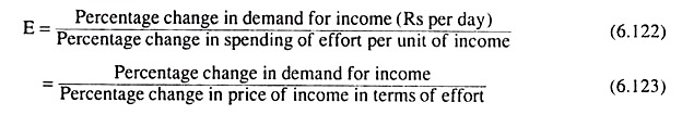
Here E is negative since the demand for income and price of income in terms of effort (labour) has been assumed to be inversely related, like all price-demand relations (barring exceptions). In Fig. 6.92, we have measured leisure (hours per day) along the vertical axis, OK or 24 hours is the maximum amount of leisure that an individual might enjoy per day, and we have measured money income (Rs per day) along the horizontal axis.

Now, if the worker does not take any income, he may enjoy the maximum amount, i.e., OK (24 hrs.) of leisure per day, and if he does not enjoy any leisure, i.e., if he wants to work 24 hrs. per day, then how much income he would be able to earn would depend upon the rate of wage per hour (W) which is the same as the price per hour of leisure (P_L).

If the rate of wage or P_L is OL₁/OK, then the consumer would be able to earn OL₁ amount of income when he enjoys no leisure. In that case, his budget line would be KL₁ in Fig. 6.92. This line would pass through the leisure- income combinations that are available to him.

The reciprocal of the numerical slope of this line, i.e., OL₁/OK, would represent the rate of wage. On the other hand, this line shows us that to earn OL₁ amount of income, the individual would have to spend efforts of OK (24) hours, and, therefore, to earn each unit of income, he would have to spend OK/OL₁ (hrs.) of efforts.

Therefore, the price of income in terms of efforts is equal to the numerical slope of the budget line, OK/OL₁. In other words, the rate of wage and the price of income (p_I) in terms of efforts are reciprocal to each other.

In Fig. 6.92, the preference-indifference pattern of the individual between income and leisure is given by the indifference curves between income and leisure. As we have already obtained, these ICs possess the usual properties of the indifference curves.

Now, if the budget line of the consumer is KL₁, i.e., if W = OL₁/OK and p_I = OK/OL₁ the individual would be in equilibrium maximising his level of satisfaction at the point of tangency E] between the budget line and one of his ICs, viz., IC₁. Let us now suppose that W increases to OL₂/Ok (OL₂ > OL₁), and p_I diminishes to OK/OL₂, giving us the budget line, KL₂, of the individual. This budget line KL₂ will be flatter than the initial budget line as its numerical slope OK/OL₂= p_I is smaller than that of the initial budget line. As a result, the individual’s equilibrium point moves from the point E₁ on IC₁ to the point E₂ on IC₂.

Now, since E₂ lies downward towards right of E₁ i.e., E₁E₂ segment of the price-consumption curve (PCC) is downward sloping to the right, the individual’s demand for income rises from OB₁ to OB₂, and his demand for leisure falls from OH₁ to OH₂, i.e., his expenditure of effort or supply of labour rises from KH₁ to KH₂, as W rises and p₁ falls.

Therefore, what we have obtained here is that as p₀ falls and the individual’s demand for income rises, his expenditure on income in-terms of effort, or, supply of labour rises. Since the price of income (p₁) and expenditure on income move in opposite directions, we obtain here e > 1, where e is the numerical value of E as defined in (6.122). Therefore, if the PCC for changes in Pi is downward sloping and e > 1, then as p_t falls and W rises, supply of labour will increase giving us a positively sloped supply curve of labour.

Let us now suppose a further fall in p_l or, a rise in W, other things remaining the same. The budget line again would become flatter, it would be, let us say, the line KL₃. As a result, the individual’s equilibrium point now would be E₃—it would move from the point E₂ on IC₂ to E₃ on IC₃.

Here it has been assumed to be a horizontal movement, i.e., here the E₂E₃ segment of the PCC has been a horizontal line. Now as p_I falls and as the equilibrium point of the indi­vidual moves horizontally from E₂ to E₃, his demand for income rises from OB₂ to OB₃ but his demand for leisure will remain unchanged at OH₂ = OH₃, i.e., his expenditure of effort or supply of labour will remain unchanged at KH₂ = KH₃.

This gives us e to be equal to one (e = 1), since as p_I falls, the expenditure on income remains unchanged. That is, if the PCC curve for changes in p_I is a horizontal straight line and e = 1, then as p_I falls and W rises, the supply of labour will remain unchanged, giving us a vertical supply curve of labour of the individual.

Lastly, if p_I falls further, i.e., W rises further, other things remaining constant, the budget line again would become flatter—it would be, let us say, the line KL₄. The individual’s equilibrium now would be E₄ on IC₄. Here the equilibrium point has moved upward towards right from the point E₃ to the point E₄, i.e., the PCC curve through E₃ and E₄ has been upward sloping.

Now as P_I falls and W rises, the person’s demand for income has increased from OB₃ to OB₄, and his demand for leisure has also increased from OH₃ to OH₄ and his expenditure in terms of effort, i.e., his supply of labour has decreased from KH₃ to KH₄.

Since the price of income and expenditure on income has moved in the same direction, here we would have e < 1. Therefore, if the PCC for changes in p_I is upward sloping and e < 1, then as p_I falls and W rises, supply of labour will decrease, giving us a negatively sloped supply curve of labour for the individual.

We may conclude that the shape of the supply curve of labour of an individual worker can be explained with the help of the concept of elasticity of demand for income in terms of effort. Like all elasticities of demand, this elasticity also will be negative. We have denoted the numerical value of the coefficient of this elasticity by e.

We have seen that (i) if e > 1, i.e., if the change in demand for income (D_I) is proportionately more than the change in the price of income (p_I), the individual supply curve of labour will be positively sloped; (ii) if e = 1, i.e., if the change in D_I is proportionate with change in p_l5 the supply curve will be vertical; and (iii) if e < 1, i.e., if change in D_I is proportionately less than the change in p_I, the supply curve of labour will be negatively sloped or backward-bending. All these points have been illustrated in Fig. 6.93.

Income and Leisure—a Mathematical Illustration:

If an individual worker’s income comes from the payment for his labour, then the optimum amount of labour supplied by him can be derived from the analysis of utility maximisation. We may also derive his demand curve for income from this analysis. Let us assume that the indi­vidual’s utility level depends on income and leisure. Then his utility function would be

U = g (L, y) (6.124)

where L and y denote amounts of leisure and income, respectively. Both income and leisure are desirable (more-is-better) goods. Here income stands for all the goods other than leisure, to be purchased by the consumer at constant prices.

Now the marginal rate of substitution (MRS) of leisure for income is

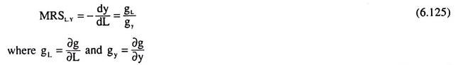
Let us denote the amount of work performed by the consumer per day by L* and the rate of wage by W.by definition,

Where T is the total amount of available time per day. The consumer’s budget constraint is

Substituting from (6.126) and (6.127) into (6.124), we obtain

To maximize U, we have to set the derivative of U w.r.t. L* equal to zero:

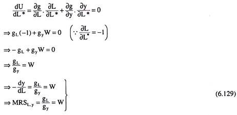
Therefore, the first-order condition (FOC) for U-maximisation states that the MRS_L,_y should be equal to the rate of wage (w).

The second-order condition (SOC) states:

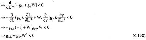
Eqn. (6.130) gives us the SOC for maximisation of utility as given by (6.124).

Equation (6.129) is a relation in terms of supply of labour (L*) and the rate of wage (W) and is based on the individual worker’s optimising behaviour. It, therefore, gives us his labour supply curve. From this relation we would be able to know the individual’s supply of labour at each W. Since demand for income is another side of supply of labour, (6.129) indirectly pro­vides us with the individual’s demand curve for income.

Example:

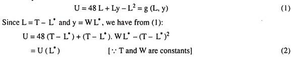
If we are given the utility function of a consumer defined for a time period of one day as:

U = 48 L + Ly – L², then we may find his utility-maximising values of supply of labour and income in the following way:

The utility function is

The first-order condition for utility maximization gives us

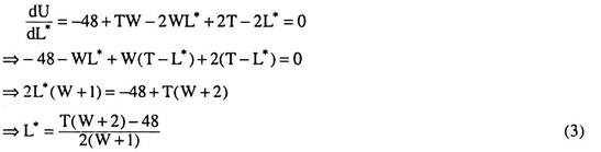
If we put the value of W and T (= 24hrs.) in (3), we would have the valu for supply of labour (L*) in hours/day. Also y may be obtained by putting the value of L* in y = WL*.

The second-order condition is also satisfied, since,

In the present example, the individual’s labour supply function has the following character­istics:

(a) Since T, the total available time is 24 hours, it is obtained from (3) that L* = 0 at W = 0, i.e., at a zero wage rate, the individual will not work at all.

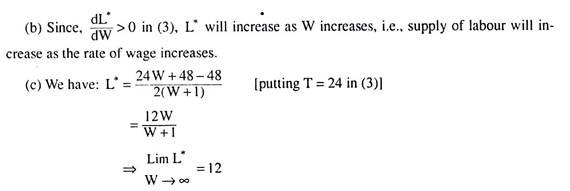
It follows then that, in this example, the individual will never work more than 12 hrs. per day however high the rate of wage may be.