Derivation of Demand Function | Consumer

In this article we will discuss about the derivation of ordinary demand function and compensated demand function.

Ordinary Demand Function:

A consumer’s ordinary demand function, is also known as the Marshallian demand function, can be derived from the analysis of utility-maximisation.

Let’s assume that the utility function of the consumer is:

U = q₁q₂                                                                                             (6.45)

And his budget constraint is:

y° = p₁q₁ + p₂q₂                                                                               (6.46)

The relevant Lagrange function needed for deriving the conditions for utility maximization is:

V = q₁q₂ + λ (y°− p₁q₁ – p₂q₂ ) (6.47)

The first-order condition for constrained utility-maximisation is:

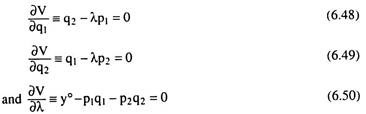
Now solving equations (6.48) – (6.50) for obtaining the equilibrium values of q₁ and q₂.

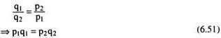
From (6.48) and (6.49), we have:

From (6.50) and (6.51), we have:

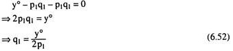
Similarly, we would have:

q₂ = y°/2p₂                                                                            (6.53)

(6.52) and (6.53) gives us the demand functions for the two goods, respectively.

Two important properties of the demand functions that is derived from above are:

(1) The demand for any commodity is a single-valued function of prices and income, For example, in eqn (6.52), it is found that for every given pair of the values of y° and p₁, having a unique value of q₁. Similarly, equation (6.53) would give a unique value of q₂ for every given pair of values of y° and p₂.

(2) The demand functions are homogeneous of degree zero in prices and income. That is, if the prices of the goods and the money income of the consumer increase (or decrease) by a certain proportion, the consumer’s demand for the goods would remain unchanged.

Compensated Demand Function:

If there is a change in the price of a commodity that the consumer purchases and if the consumer is duly compensated for the price change, i.e., if he is taxed after a fall in price or subsidized after a rise in price to such an extent that his level of utility remains the same, then his price-demand relation for the commodity is known as his compensated demand function for the good.

In order to derive such a function let’s assume that the utility function of the consumer is:

U = q₁q₂                                                                                  (6.54)

And his budget equation is y^o = p₁q₁ + p₂q₂           (6.55)

Under the ‘compensated’ conditions, the consumer would purchase such a combination of the goods that would minimise his expenditure for the goods subject to the utility constraint:

U^o =q₁q₂                                                                                 (6.56)

where U^o is the utility level at his initial equilibrium point.

Here the relevant Lagrange function is:

V = p₁q₁ +p₂q₂ + µ (U^o − q₁q₂) (6.57)

The first-order conditions are given by:

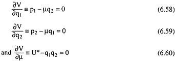
From (6.58) and (6.59), we have:

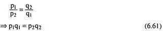
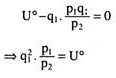
From (6.60) and (6.61), we have:

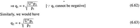
Eqns. (6.62) and (6.63) gives the consumer’s compensated demand functions for the two goods. It is evident in these demand functions that if there are proportionate changes in pi and p₂, the consumer’s demand for the goods, i.e., qi and q₂, would remain unchanged. In other words, the compensated demand functions are homogeneous of degree zero in the prices of the goods.