Some Pathological Demand Curves (With Diagram)

Some Pathological Demand Curves:

Normally, the demand curve of an individual for a certain good slopes downward towards right because of the income effect and the substitution effect of a change in its price. But in some cases, we may have abnormal or ‘pathological’ demand curves.

One such case is the case of a Giffen good. Sometimes, it is observed in the case of a good, say, X, that, initially, the nature of the income effect is such that along with the substitution effect, the demand curve would be sloping downward towards right as the price of the good falls and the consumer’s real income rises.

But after a certain point, say, E in Fig. 6.60, the good becomes a Giffen good, i.e., the nature of the income effect for the good becomes so ‘abnormal’ that it overpowers the normal behaviour of the substitution effect and makes the demand curve slope downward towards left with the successive falls in the price of the good and the consequent rises in the consumer’s real income.

Therefore, the individual’s demand curve, d_x, in the Giffen good case would have a kink at the point E in Fig. 6.60. It may be noted here that the abnormality of the demand curve in the Giffen good case is not because of any relaxation of the axioms of ordinal utility.

It is obtained in spite of the ICs being convex to the origin. It occurs because, after a point, the preference pattern of the consumer makes the good ‘strongly’ inferior to him vis-a-vis other goods, although the good remains an MIB.

There may, however, be some other pathological cases that may be obtained because of departure from the axioms of ordinal utility. One such case is obtained when the individual’s IC is convex for some parts of its length and concave elsewhere, i.e., it is not convex (to the origin) everywhere. Two such curves have been shown in Fig. 6.61.

If the budget line of the consumer is A₁B₁, IC₁ is the highest IC that the consumer can reach, but not at a unique point. He may stay at any one of the two points on IQ, viz., E and G. He cannot choose the point F on IC₁, because, F lying on a higher budget line A₂B₂, would require a larger amount of money that would enable the consumer to reach the point H on a higher IC, viz., IC₂.

Therefore, given the shape of the ICs in Fig. 6.61, any budget line, say, A₂B₂, can touch two ICs—at a concave section of the lower curve, IC₁ at the point F, and at two convex sections of the higher curve, IC₂ at the points H and L.

Let us now suppose that the price of good X implicit in the parallel budget lines A₁B₁, A₂B₂, etc., is p_x⁽²⁾ , and the consumer’s income implicit in the budget line A₂B₂ is M₂. Given his income and the price of X, his budget line will be A₂B₂, and the quantity purchased of good X would be x₁ at the point H, or, x₂ at the point L.

In other words, we have obtained here that at the price p_x⁽²⁾, demand for X may be x₁ or x₂. Since at the price of p_x⁽²⁾, the consumer cannot demand any quantity that lies between x₁ and x₂, there would be a horizontal discontinuity in the demand curve for good X at the price p_x⁽²⁾.

The pathological demand curve, d_x, in this case would be like the curve shown in Fig. 6.62. It would be a curve in two parts, viz., MN and RS, and, there would be a discontinuity between these two parts at the price p_x⁽²⁾.

Lastly, we shall discuss a pathological case where the demand curve would have a vertical section like that of the demand curve, d_x in Fig. 6.63(b). This type of demand curve would be obtained if the indifference curve has any ‘sharp’ corner such as A in Fig. 6.63(a).

The peculi­arity of this case lies in the fact that each of an array of prices, say, p_x⁽¹⁾, p_x⁽²⁾, p_x⁽³⁾,… of good X implicit in the budget lines H₁, H₂, H₃,… will give us the same equilibrium of the consumer at the point A.

In other words, at all these prices, viz., p_x⁽¹⁾, p_x⁽²⁾, p_x⁽³⁾,… the equilibrium quantity demanded of good X will be the same, say, x₀, and so over the range of these prices the consum­er’s demand curve for good X would have a vertical section.

Nonlinear Budget Lines:

In the indifference curve theory, if the prices of the two goods, X and Y, are given and constant w.r.t. their quantities purchased, the consumer’s budget line will be linear—it will be a nega­tively sloped straight line.

Now, if the prices are not constant, then we would get non-linear budget lines in place of the linear ones. For example, let us suppose that the consumer has the market power such that he can buy more of a good, say, X, at a smaller price, the price of the other good (Y) remaining the same irrespective of the quantity he purchases.

In this case, as the consumer buys more of good X, p_x falls, p_Y remaining unchanged, and so, p_x/p_y would fall. That is, the numerical slope of the budget line would fall as the consumer buys more of X, i.e., the budget line would be flatter downwards, or it would be convex to the origin, like the curve AB in Figs. 6.64-6.66.

If the indifference curves (ICs) are of usual shape, i.e., if they are negatively sloped arid convex to the origin, then consumer equilibrium solution would be a corner solution either at the corner A in Fig. 6.64, or, at the corner B in Fig. 6.65, depending on whether the ICs are flatter or steeper throughout than the budget line.

But if the ICs are parallel to the budget line wholly or partially like the ICs in Fig. 6.66, then one of these ICs would coincide wholly or partly with the budget line. This has happened in Fig. 6.66, in which the curve IC₃ has coincided with the budget line over the stretch RS.

In this case, we would not obtain a unique equilibrium solution. For, any point on this stretch would be an equilibrium solution—it would lie on the budget line and also on the highest possible IC (here IC₃).

Lastly, the consumer’s budget line would be non-linear and concave to the origin if he has monopsonistic power in the market, i.e., if the price of good X rises as the consumer buys more of X, the price of good Y remaining unchanged irrespective of its quantity purchased.

Here as the consumer buys more of X, i.e., as he moves downward towards right along his budget line, p_X/p_Y rises, i.e., the numerical slope of the budget line rises. In other words, here the budget line would be steeper downwards or it would be concave to the origin like the budget line AB in Fig. 6.67.

Now if the ICs are negatively sloped and convex to the origin, then here we would get a unique and interior equilibrium solution at the point of tangency between the budget line and an IC. This equilibrium solution is given at the point T in Fig. 6.67. At this point, the consumer would buy OM of good X and ON of good Y.

It may be noted here that if only the money income of the consumer rises, the convex or concave budget line would shift upwards or to the right, but its slope (p_x/p_y) would remain the same at each x, because, at each x, p_x would be the same for each budget line (while p_Y remains unchanged by assumption).

The students may verify for themselves whether the analysis relating to the effects of price and income changes in the corner and interior (point of tangency) solution cases can be applied to the cases.

Example 1:

If an individual’s utility function for two goods is given by U = x^αy^β and if the individu­al’s budget constraint is given by M = p_x.x + p_y.y, derive his individual demand functions for the goods X and Y in terms of M, α and β.

Solution:

The individual’s utility function is

U = x^αy^β (1)

and his budget constraint is

M = p_x.x + p_y.y (2)

where M is his fixed income.

The utility-maximising individual’s demand functions for the goods have to be derived from the conditions for utility maximisation.

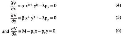
In order to obtain these conditions, let us form the relevant Lagrange function:

From (3), we obtain the first-order conditions for constrained utility maximization to be:

Dividing (4) by (5) after transposing the terms, we obtain:

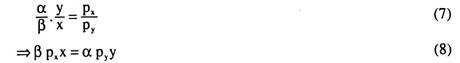
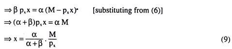
Again, from (6) and (8), we obtain:

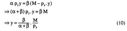
(9) and (10) give us the required demand functions of goods X and Y in terms of M, a and p.

Example 2:

Given an individual’s utility function U = (x + 2) (y + 1), prices p_x = 2 and p_y = 6, and income M (X and Y being the two commodities on which the individual spends his entire income),

(a) Write the relevant Lagrange expression and explain its rationale;

(b) Find the individual’s demand for X and Y;

(c) Check that the second-order conditions are fulfilled;

(d) What do the second-order conditions mean in economic terms?

Solution:

We are given the utility function of the consumer as:

U = (x + 2) (y + 1) (1)

and his budget line is:

M = p_xx + p_yy

or, M = 2x + 6y (2)

where M is the given amount of his income.

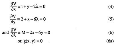
(a) The relevant Lagrange function for utility-maximisation subject to budget constraint is:

V = (x + 2)(y+ 1) + λ(M-2x-6y) (3)

The Lagrange function (3) is so constructed that if the constraint is satisfied, V becomes identical with U. Therefore, the conditions for maximisation of V give us the conditions for maximisation of U subject to the budget constraint.

Here lies the rationale for forming the Lagrange function. We may also observe that maximisation of V guarantees that the budget constraint (2) would be satisfied, since the first-order conditions for such maximisation include M – p_xx – p_yy = 0 [eq. (6)].

(b) The first-order conditions for constrained maximisation of U are:

As noted, condition (6) gives us that the budget constraint (2) is satisfied.

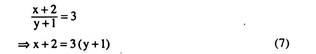
Dividing (5) by (4), after suitable transposition of terms, we have:

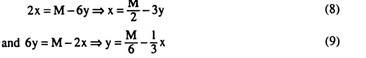
Now, from (6):

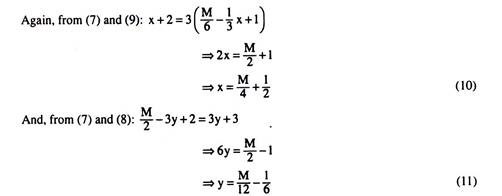
The individual’s demand for x and y are given by (10) and (11), respectively.

(c) The second-order condition gives us:

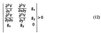
Now, putting the value from (4), (5) and (6a), the left hand side of (12) is obtained to be:

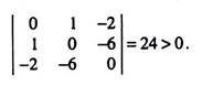
Therefore, it is verified that the second order condition is fulfilled.

(d) The second-order condition helps us to establish that the indifference curves (ICs) would be convex to the origin at the point where the first-order conditions are satisfied, i.e., at the point of tangency between the budget line and an IC. The economic significance of this is that the marginal rate of substitution of x for y would be diminishing as the consumer substitutes x for y.

Example 3:

(i) Find the optimal levels of commodity purchased for a consumer whose utility function and budget constraint are V = q₁^1.5 q₂ and 3q₁ + 4 q₂ = 100, respectively.

(ii) Show that the optimal bundle would remain the same if his utility function was:

V = 1.5 log q₁ + log q₂. Does this result seem puzzling to you? Explain your answer.

Solution:

(i) The utility function of the consumer is:

and his budget constraint is:

For finding the optimum commodity bundle, we have to construct the relevant Lagrange function:

The first-order condition for utility maximization subject to the budget constraint are:

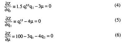
Dividing (5) by (4) after suitable transposing the terms:

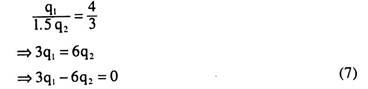
Adding (6) and (7):

Putting q₂ = 10 in (7):

Therefore, the optimum levels of purchase are q₁ = 20 units and q₂ = 10 units, assuming that the second-order condition is satisfied, (ii) The utility function now is

W = 1.5 logq₁ + logq₂ (8)

[We have used the notation W in place of V because this is a different utility function than (1)].

The budget constraint is the same as (2),

For finding the optimal levels of the goods, the relevant Lagrange function is

T = 1.5 log q₁ + log q₂ + λ (100 – 3q₁ – 4q₂)

The FOCs are obtained as:

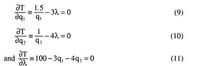
From (9) and (10), we have

Since (11) and (12) are the same as (6) and (7), the solutions for optimum levels of the goods would be the same as have been obtained before in (i), i.e., q₁ = 20 units and q₂ = 10 units assuming that the SOC is satisfied.

The result that we obtain the same optimal levels for the goods for two different utility functions (1) and (8) does not seem puzzling to us because the utility function (8) is a positive monotonic transformation of (1).

This may be seen as follows:

where V is the utility function (1)

Now, W = F(V) is a positive monotonic transformation of V since F(V₁) > F(V₀) whenever V₁ > V₀. The utility function obtained by means of positive monotonic transforma­tion of another utility function represents the same utility index and indifference map, and, therefore, the same optimal point as the original function,

Example 4:

Under what conditions would it be possible for a consumer to be in equilibrium:

(a) While the marginal utilities (MUs) of some goods he consumes are zero?

(b) While the MUs of some goods he refuses to buy are greater than the MUs of some goods he does purchase?

(c) While the MUs of all goods he purchases are exactly proportional to their prices?

(d) While the MUs of all the goods he purchases are exactly equal?

Solution:

In order to be able to use the indifference curve (IC) theory, we shall assume here that the consumer buys only two goods X and Y.

(a) Let us suppose, MU_X = 0 and, by the usual MIB assumption, MU_Y > 0.

Therefore, MRS_X,_Y = MU_X/MU_Y = 0

=> The numerical slope of the ICs = 0

=> The ICs would be horizontal straight lines.

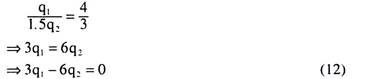
If the ICs are horizontal straight lines, the consumer is able to reach the highest possible IC at the corner point of the budget line with the y-axis in Fig. 6.68. In other words, here we would have a corner solution, and at the equilibrium point A, the nothing of good X.

The economic interpretation of the nature of consum­er’s equilibrium that we have obtained in this case is very simple. Since MU_X = 0 and MU_Y > 0, we obtain MU_X = 0 and

MU_Y > 0, i.e., the MU of money spent on good X is zero and the MU of money spent on good Y is positive. Since the MU of money spent on good X is zero, the consumer spends nothing on this good and buys noth­ing of it.

Therefore, he has to spend all his money on good Y and he buys OA of good Y as seen in Fig. 6.68, and since the MU of money spent on Y is positive, he has no difficulty in spending all his money on good Y.

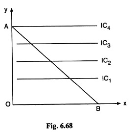
However, if we assumed just the opposite, i.e., MU_X > 0 and MU_Y = 0, then the numerical slope of the IC would be MU_X/MU_Y = ∞, i.e., the ICs would be vertical straight lines as shown in Fig. 6.69. In this case, the consumer can reach the highest possible (i.e. furthest from the ori­gin) IC along the budget line at the point B.

Here also we have a corner solution. But now the consumer will buy only good X (OB of good X) and nothing of Y. For now the MU of money spent on good X is positive (MU_X/p_x > 0) and the MU of money spent on good Y is zero (MU_Y/p_y = 0)

(b) Let us assume (according to the given conditions) that the consumer purchases only good X and refuses to purchase Y although MU_X < MU_Y.

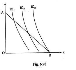
Now, he may purchase only X if equilibrium takes place at the corner B of his budget line AB with the x-axis in Fig. 6.70. If we assume that the ICs possess their usual properties, i.e., if the ICs are negatively sloped and convex to the origin, then a corner solution at point B may be obtained when the ICs are steeper everywhere than the budget line as shown in Fig. 6.70. Now,

good X is greater than the MU of money spent on good Y everywhere along the budget line.

It follows from above that equilibrium at point B requires:

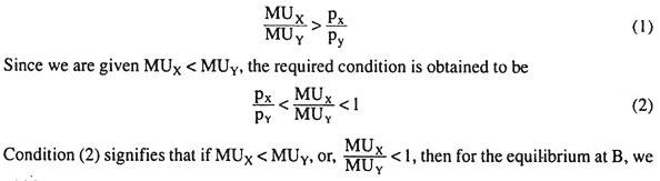
should have not only p_x/p_Y < MU_X/MU_Y, but also p_x/p_Y < 1, or, p_x < p_Y. This, in its turn, signifies that if MU_x/MU_Y, or, the marginal significance of X in terms of Y is less than 1 (one), then p_x/p_Y, or, the market price of X in terms of Y should not only be less than 1 (one), but also it should be less than the marginal significance of X in terms of Y.

Only then the consumer will buy only X and no Y, even if MU_X < MU_Y. (c) We are given, at any point on an IC:

i.e., numerical slope of an IC = numerical slope of the budget line = constant (given p_x and P_y).

This implies that the ICs are negatively sloped straight lines and parallel to the budget line. In this case, the consumer would be in equilibrium at any point on the IC that happens to coincide with the budget line,

(d) We are given:

MU_X = MU_Y (4)

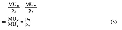
Assuming that the ICs possess their usual properties, the consumer’s equilibrium condition gives us

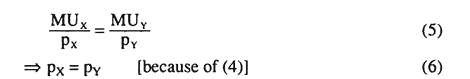
Therefore, if MU_X = MU_Y, then the consumer would be in equilibrium at the point of tan­gency between his budget line and one of his ICs if p_x = p_Y.

Example 5:

A consumer in a two commodity world has indifference curves with a slope = 0.5 everywhere. Find his equilibrium purchase plan when price of X (p_x) = Rs 5, price of Y (p_Y) = Rs 5 and his planned expenditure is Rs 1,500. What happens when p_x = Rs 3 and p_Y = Rs 6.

Solution:

We are given the following information:

(i) Price of X (p_x) = Rs 5, then changes to Rs 3

(ii) Price of Y (p_Y) = Rs 5, then changes to Rs 6

(iii) Planned expenditure of the consumer (M) = Rs 1,500

(iv) The numerical slope of the ICs = 0.5 everywhere

i.e. the ICs are negatively sloped straight lines of slope = – 0.5.

From the above data, we obtain that the numerical slope of the budget line is P_X/P_Y = Rs5/Rs 5 = 1whereas the numerical slope of the straight-line ICs are 0.5. So, here the ICs are straight lines flatter everywhere than the budget line.

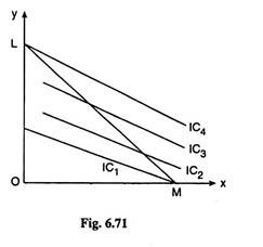
In such a case we would have a corner solution at the point where the budget line meets the y-axis. That is, the equilibrium purchase plan of the consumer would be zero of X and Rs 1,500/ Rs 5= 300 units of y—he would purchase only y. The solution is obtained at the corner point L of the budget line LM in Fig. 6.71.

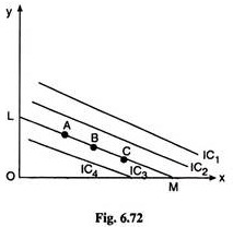
In the second case, the numerical slope of the budget line is p_X/p_Y= Rs 3/ Rs 6 = 0.5 and the nu­merical slope of the straight line ICs is also 0.5, i.e., here the ICs would be parallel to the budget line. In such a case, the consumer would be in equilibrium at any point like A, B, C, etc. that lie on the IC, viz., IC₃, which coincides with the budget line LM in Fig. 6.72. Here no unique equilibrium solution would be obtained.

Example 6:

What does it mean if a consumer’s indifference curves are negatively sloped, with higher indifference curves showing lower level of utility?

Solution:

Let us assume that the utility function of the consumer is

U = f(x,y)                (1)

Taking total differential of (1), we get

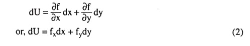
Now, for a movement along an IC, we have, dU = 0. So (2) gives us

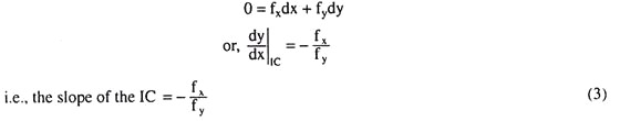
From (3) we obtain that the slope of the IC may be negative if:

(i) Both f_x (= MU_X) and f_y (= MU_y) > 0. i.e., if both the goods are ‘goods’, i.e., they are of “more is better” (MIB) type, or, (ii) both f_x (= MU_X) and f_y (= MU_y) < 0 i.e. if both the goods are ‘bads’, i.e., they are of “more is worse” (MIW) type.

In case (i), a higher IC represents a higher level of satisfaction, for any point on a higher IC like the point A on IC₂ in Fig. 6.73, may be shown to represent a combination of more of both the goods than some point like B on the lower IC, viz., IC₁. Since MU_X, MU_y > 0, utility-level at A here is higher than the utility level at B.

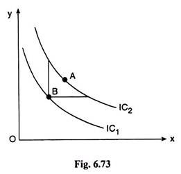
On the other hand, in case (ii), a higher IC would rep­resent a lower level of satisfaction. For, now, since MU_X, MU_Y < 0, the point A on the higher IC, viz., IC₂, repre­senting more of both the goods, would give the consumer a lower level of satisfaction than point B on the lower IC which is IC₁.

We may conclude, therefore, that in the case of nega­tively sloped ICs, the higher curve representing a lower level of satisfaction, implies that both the goods are of “more is worse” type, i.e., MU_X, MU_Y < 0.

Example 7:

(a) Take any two points on a normally shaped indifference curve and join them by a straight line. What does the slope of this line indicate?

(b) What is the significance of an indifference curve with a segment parallel to the vertical axis?

(c) Prove that, at any point on a budget line, the line can cut or touch only one indifference curve.

Solution:

(a) Let us suppose that the consumer buys only two goods, X and Y, and the normally shaped indifference curves of the consumer for X and Y is given to us.

Now the numerical slope of the straight line obtained by joining any two points on an IC would give us the rate of substitution of X for Y on average over the arc of the IC between the two points (the consumer’s level of satisfaction remaining constant).

However, if the two points are sufficiently close to each other so that the straight line joining them may become a tangent to the IC, then the numerical slope of the tangent would represent what is called the marginal rate of substitution of X for Y.

It may be noted here that MRS of X for Y at any point on an IC is defined as the quantity of Y that the consumer is willing to forego for obtaining an additional unit of X, provided his level of satisfaction remains constant.

Let us now illustrate the point under discussion with the help of Fig. 6.74. In Fig. 6.74, any two points on an IC are P and Q. The numerical slope of the straight line joining these two points is PT/TQ. Now what PT/TQ represents would be clear to us if we think like this.

As the consumer moves from the point P to the point Q, he is giving up PT of Y and taking in TQ of X. So for getting each additional unit of X, he has to forego, on average, PT/TQ of Y. So PT/TQ is the av­erage rate of substitution of X for Y over the arc PQ of the IC concerned.

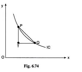
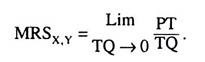
On the other hand, the limiting value of PT/TQ as P o approaches Q along the arc PQ or as TQ → 0, gives us MRSX,Y i.e., we have

(b) We are given that the IC of a consumer has a segment parallel to the y-axis. If we assume that the rest of the curve is normally shaped, then the IC would look like the one drawn in Fig. 6.75 below.

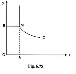
In Fig. 6.75 the segment of the IC below the point M is normally shaped. That is, along this segment, both x and y are goods of “More is better (MIB) type”. But the IC becomes parallel to the vertical axis above the point M.

Along this vertical segment, given the quantity of x (OA), more of y does not increase (or decrease) the level of satisfaction of the consumer. In other words, along the vertical segment, the marginal utility of Y becomes equal to zero.

Therefore, if the IC is like the one given in Fig. 6.75, then more of Y is welcome to the consumer up to a certain quan­tity (here OB). If the consumer has more of Y beyond this point, marginal utility of Y becomes equal to zero, i.e. Y remains no longer an MIB good to the consumer. It may be noted, however, that for such an IC, X is always an MIB good.

We may also mention here that, along the vertical segment of the IC, its numerical slope is infinitely large, and so the MRS_X,_Y is also equal to infinitely large along this segment. This is also clear from the fact that MRS_X,_Y = MU_X/MU_Y, and when MU_Y = 0, MU_X,Y = ∞.

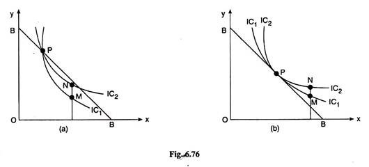
(c) At any point on the budget line, the line can cut or touch only one IC. Because, if at any point on the budget line, the line cuts or touches more than one IC, as shown in Fig. 6.76, then these ICs would cut or touch each other at that point. But one of the standard properties of the ICs is that they cannot cut or touch each other.

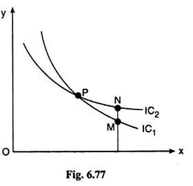
Let us now see, what happens if any two ICs cut or touch each other. In Fig. 6.77, the two ICs have cut each other at the point ‘P’.

Let us take any point M on IC₁ and the point N on IC₂, such that N is vertically above M. Now the consumer is indifferent between M and P, for both of them lie on IC₁. Again, the consumer is indifferent between P and N, for both of them lie on IC₂. Therefore, under the transitivity condition, he is indifferent between M and N.

But he can­not be indifferent between M and N because of the MIB assumption, for N has more of Y but the same quantity of X as M. So if any two (or more) ICs cut each other at a point, we arrive at a logical contradiction. The same thing would happen if the ICs touch each other.

Now since the ICs cannot cut or touch each other, it is not possible for the budget line to cut or touch more than one IC at any point on it.

Example 8:

Consider a consumer in a two-commodity (X and Y) world whose indifference map is such that the slope of the ICs is everywhere equal to –x/y , where x and y are the quantities of X and Y, respectively.

Show that the demand for X is independent of the price of Y and the price-elasticity of demand for X is unitary.

Let us suppose that the prices of goods X and Y are p_x and p_Y, respectively. By the given condition the MRS_X,_Y = y/x

At the point of consumer equilibrium

MRS_{X Y} = p_x/p_y (1)

From (1) and (2), we have

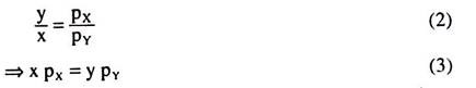
It is obtained from (3) that the consumer spends half of his money income (M) on X irre­spective of p_Y, and half on Y. This gives us that the demand for X is independent of p_Y.

Now, if M remains constant, we have

Taking total differential of (3), we have

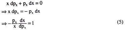
Since the coefficient of price-elasticity of demand is

(4) gives us E = − 1

and the numerical coefficient of price-elasticity of demand is 1.

Example 9:

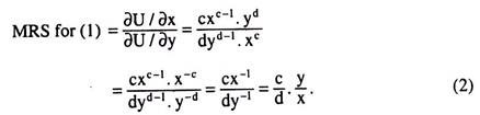
Derive the MRS for the Cobb-Douglas utility function and that for a positive monotonic transformation of the function, and comment on the result.

Solution:

Let us suppose that the Cobb-Douglas utility function is

By definition, we have

Let us now derive the MRS for a positive monotonic transformation of (1), which is taken to be

Where v is the monotonically transformed utility from U.

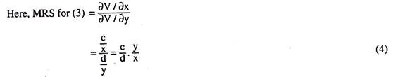
We have obtained the MRS for the two cases as given by (2) and (4), to be identical. This is because the positive monotonic transformation of a utility function represents same prefer­ences as the original function.

Example 10:

Derive the Cobb-Douglas Demand Functions from Cobb-Douglas Utility Function Let us suppose that the Cobb-Douglas utility function is given as

U (x, y) = x^cy^d                 (1)

and the budget constraint of the consumer is

M = p_x x + p_yy                 (2)

Since the utility function (1) is the same as any of its positive monotonic transformation, let us replace (1) by

log [U (x, y)] = c log x + d log y                    (3)

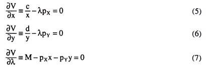
Let us now maximise the utility function (3) subject to the budget constraint (2). The relevant Lagrange function is

V = c log x + d log y + λ (M – p_xx – p_yy)           (4)

Now, the first-order conditions for the required maximum are:

Equation (7) just gives us that the constraint (2) is satisfied and from equation (5) and (6), we have

Adding (8) and (9), we have

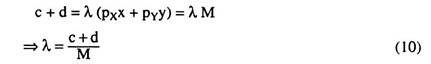
Now, from (8) and (10), we have

Similarly, from (9) and (10), we have

The required Cobb-Douglas demand functions for goods X and Y are given by (11) and (12).

Example 11:

Derive the demand function for quasi-linear preferences.

Solution:

Let us suppose that the quasi-linear preferences are represented by the following utility function:

U (x, y) = V (x) + y                     (1)

and the budget line of the consumer is given by

M = p_xx + p_Yy                             (2)

In order to derive the required demand function, we have to maximise U in (1) subject to the budget constraint (2).

Let us solve the budget constraint (2) for y as a function of x, and obtain

Substituting from (3) in (1), we have the constrained utility function as

Now, the first-order condition for constrained maximization of U is

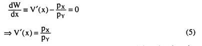
Eqn. (5) gives us the required demand function for good X. This demand function has the interesting feature that the demand for good X must be independent of income. [This is nothing new to us. We also came to know about this in our indifference curve analysis of consumer equilibrium under quasi-linear preference.]

From (5), we may write the inverse demand function for good X as

Px(x) = V'(x) p_Y                                             (6)

That is, the inverse demand function of good X is the partial derivative of the utility function w.r.t. x [^._.^. V'(x) = ∂_U/∂_X] multiplied by p_Y. Once we have the demand function for good X, the demand function for good Y is obtained by putting the value of x obtained from (6) in the budget constraint (2).

Example 12:

Derive the demand functions for the quasi-linear utility function, U (x, y) = log x + y.

Solution:

The utility function of the consumer is given to be:

U (x, y) = log x + y                     (1)

Let us suppose that his budget constraint is

M = p_xx + p_Yy                             (2)

In order to derive the required demand functions, we have to maximise U in (1) subject to the budget constraint (2). From (2), we obtain

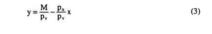
Substituting from (3) in (1), we have the constrained utility function as

Now, the first-order condition for constrained maximization of U is

Eqn. (5) gives us the direct demand function for good X. Let us note that demand for good X is independent of the consumer’s money income, M.

From (5) we may write the inverse demand function for good X as

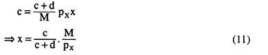
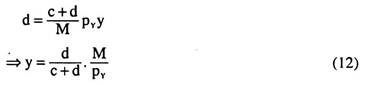
Now, putting the value of x from (5) in the budget constraint (2), we obtain

(7) gives us the direct demand function for goods Y. From (7), we obtain the inverse demand function for goods Y as

We have seen in (5) that demand for good X is independent of the consumer’s money income. Actually, from theory that in a two-good (X and Y) model of quasi-linear preference the utility function is linear in the quantity of one of the goods, say, Y and it is generally non-linear in the quantity of the other good, X.

For such a function, demand for good X becomes independent of the money income of the consumer, i.e., demand for good X remains constant as money income changes. However, this can be true only over a certain range of the value of income. A demand function cannot be independent of income for the whole range of income values.

For example, when income reduces to zero or very near zero, demand for X cannot remain constant—demand for both the goods would approach zero then.

Now, at what quantity, the demand for good X would remain constant would depend upon the slope of the budget lines corresponding to different levels of income, i.e., on the ratio of the prices of the goods. Let us suppose, that quantity of X is x₀.

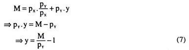
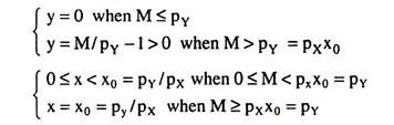
Therefore, so long as the money income (M) > p_x.x₀, the consumer would always buy x₀ of good X. In the case of utility func­tion (1), we would have x = x₀ = p_y/p_x [from (5)], given p_x and p_Y. For M < p_xx₀, his demand for X cannot remain constant at x₀.

At M = p_xx₀, he would buy x₀ of X along with zero of Y, and for M < p_xx₀, his purchase of X decreases and approaches zero along the x-axis, since y = 0. Therefore, the income-consumption curve would have two parts. The first part would be the segment of the x-axis from the origin (x = 0) to x = x₀ = p_Y/p_x and the second part would be a vertical straight line at x = x₀, for M ≥ p_xx₀.

We may now relate the demand for Y to that for X. At M = p_x x₀ = p_Y [from (5)], y = 0, since all the money would be spent on X, and at M < p_x x₀ = p_Y also, y = 0. This is because M is so small (M < p_x) that not even a single unit of Y can be purchased. Therefore, all the money now would be spent on x, though we would have x < x₀, since M < p_xx₀.

Lastly, for M > p_x x₀, as M increases x remains constant at x₀, and so M − p_x x₀, or, the money spent on Y increases and so demand for Y increases and we would have

Therefore, a better way to write the demand for the goods X and Y (assuming the utility function (1) and the prices of the goods given to be p_x and p_Y) is

Example 13:

A diminishing MRS implies that the MU of each good is diminishing. Is this statement true or false? Give reasons.

Solution:

For a two-commodity consumer, let us suppose that the ordinal utility function is

U = f(x,y)                                 (1)

Now, the MRS of good X for good Y is defined as

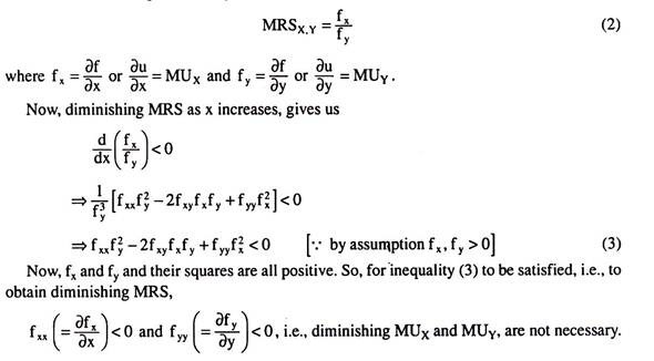
Because, positive f_xx and f_yy with a sufficiently large and positive f_xy might also satisfy (3).

Again, for diminishing MRS, diminishing MU, i.e., f_xx, f_yy < 0, is not sufficient. Because, then, a sufficiently large and negative value of f_xy might make (3) impossible. Therefore, the given statement is not true.

Example 14:

If over the relevant range, the PCC for good Y is parallel to the y-axis, then the demand curve for Y is a straight line. Is this statement true or false? Give reasons.

Solution:

Let us suppose that the two goods that are used by the consumer are good Y measured along the y-axis and money measured along the x-axis. Let us also suppose that the total quantity of money with the consumer is M and the quantity of money retained by him is m. Therefore, the amount of money spent by the consumer on Y is M − m.

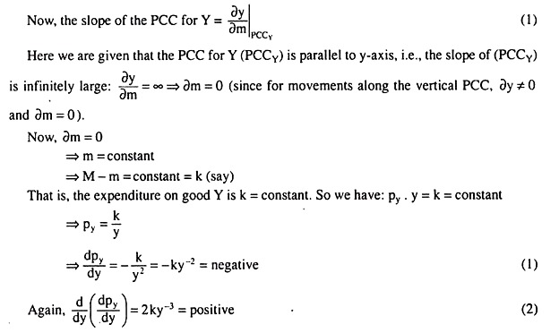
From (1) above, we may conclude that the given statement is not true. Because, we obtain

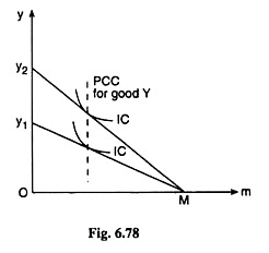
that the slope of the demand curve for good Y is negative and from (2), we obtain that the slope of the demand curve increases as y increases.

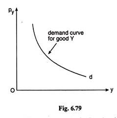
Therefore, (1) and (2) give us that the demand curve for good Y is not a straight line. It is negatively sloped and convex to the origin. The PCC for good Y as per the given conditions and the demand curve for good Y with features obtained, have been shown in the diagrams.

Example 15:

In a 2-commodity world, show that the two goods cannot be inferior simultaneously.

Solution:

The budget equation of the consumer is:

P₁q₁ + P₂q₂ = M                               (1)

where p₁ and p₂ are the prices of the two goods, and q₁ and q₂ are the quantities purchased of the two goods, and M is the consumer’s money income.

In consumer theory, it is assumed that the LHS of (1), i.e., the expenditure of the consumer, is equal to the RHS, i.e., the consumer’s money income.

Given this assumption, if both the goods are inferior, then, as M rises, p₁ and p₂ remaining constant, q₁ and q₂ both would fall, and then the expenditure of the consumer cannot be equal to his income, i.e., the budget equation would not be satisfied. Hence both the goods cannot be inferior simultaneously.

The same problem may be presented geometrically in this way. According to the assumption of the theory, the consumer must remain on his budget line, spending all his money. Let us suppose that, initially, the consumer is at the point P on his budget line A₁B₁ in Fig. 6.80.

Now, if his money income, M, rises, the prices of the goods, Pi and p₂ remaining unchanged, then his budget line would have a parallel rightward shift from A₁A₁ to A₂B₂, and the consumer, by assumption would have to remain at some point on his new budget line, A₂B₂.

In that case, the consumer would have to buy more of both the goods (at any point on A₂B₂ between R and S), or, he would have to buy more of one good and the initial quantity of the other good (at the point R or S) or he would have to buy more of one good and less of the other good at any point like E and F, on A₂B₂ other than those lying on the segment RS.

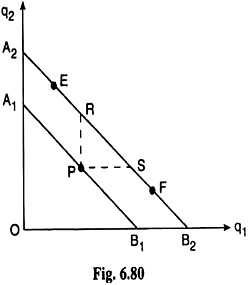
But nowhere on A₂B₂ can he buy less of both the goods, which he would be required to do if both the goods are inferior to him simultaneously. Therefore, in this two-good model both the goods cannot be inferior simultaneously.

Example 16:

While it is impossible for all goods that a consumer buys to be Giffen goods, there is no reason why they should not all be simultaneously inferior—true or false? Give reasons.

Solution:

There are two parts of the given statement. Let us first take up the first part which is:

it is impossible for all goods that a consumer buys to be Giffen goods. This statement is true, intuitively. For the sake of simplicity, we shall assume that the consumer purchases only two goods, and he has a given amount of money income all of which he has to spend, by the assumption of the theory, on the two goods.

Now, the price-demand relation for a Giffen good, is positive, i.e., if the price of the good rises (falls), the quantity demanded of the good also rises (falls). Now, if both the goods are Giffen goods, then if the prices of both of them rise, the consumer would buy larger quantities of both of them which is impossible with a given amount of money income.

Conversely, if the prices of both the goods fall, the consumer would have to purchase less of both the goods by spending less than his money income, which is also not possible by assumption. Hence, both (i.e., all) the goods purchased by the consumer cannot be Giffen goods. Therefore, the first part of the given statement is true.

We may now establish, mathematically, that the first part of the given statement is true.

For a two-commodity consumer, the budget constraint is:

M = p₁q₁ + p₂q₂                             (1)

where q₁ and q₂ are the quantities purchased of the two goods, pi and p₂ are their prices, and M is the given amount of the consumer’s money income which he has to spend on the two goods.

Taking total differential of (1), M remaining constant:

0 = p₁dq₁ + q₁dp₁ + p₂dq₂ + q₂dp₂                        (2)

Now, if all (here both) the goods are Giffen goods, we would have: dq1, dq2 ≠ 0 when dp1, dp2 ≠ 0. And, in that case, the right hand side of (2) would be either positive or negative (p1, p2, q1, q2 being > 0) while the left hand side is equal to zero, i.e., (2), and so (1), will not hold, and so all goods the consumer buys, cannot be Giffen goods. Therefore, the first part of the given statement is true.

Let us now come to the second part of the statement which is: there is no reason that all goods that a consumer buys should not be simultaneously inferior. That is, according to the statement all the goods purchased by the consumer may be simultaneously inferior.

Intuitively speaking, this statement is not true. For in the two-good case where a given amount of money income is to be spent, if both the goods are inferior and consumer’s money income increases (decreases), prices remaining constant, the consumer would buy less (more) of both the goods. In the event, he must underspend (overspend) his money.

Therefore, both (or all) the goods purchased by the consumer cannot be inferior goods, and so, the statement is not true. We shall now establish mathematically that the second part of the statement is not true. Taking the total differential of the budget constraint (1), p₁ and p₂ remaining constant, we have

dM = p₁dq1 + p₂dq₂ (3)

Now, if both the goods are inferior, we would have: dq,, dq₂ ≠ 0 when dM ≠ 0, and in that case, the right hand side of (3) would be positive or negative when the left hand side would be negative or positive, i.e., (3), and so (1), will not hold, and so all (here both) the goods purchased by the consumer cannot be inferior. Therefore, the second part of the given statement is not true. 

Example 17:

It is impossible for both an individual’s price elasticity of demand for a good and his income elasticity of demand for the same good to be simultaneously positive. Is this statement true or false. Give reasons.

Solution:

Let us assume a two-good (good X and good Y) model. Price elasticity of demand for good X is given by:

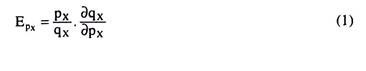
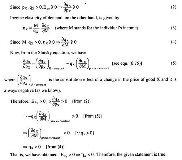
Example 18:

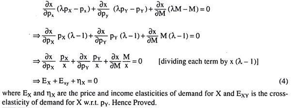
Prove that the sum of own-price, cross- and income-elasticities of demand for a commodity is equal to zero.

Solution:

The demand function for good X may be written:

x = f (p_x, py, M)                              (1)

where x = demand for good x, p_x = price of good x and p_y = price of good y and M = money income of the consumer concerned.

Since the demand function for any good is homogeneous of degree zero in prices and in­come, we have:

 

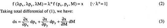
On the basis of (1), (2) and (3), we obtain

Example 19:

What is the nature of the consumer if his ICs are concave?

Solution:

Concave-to-the-origin ICs (Fig. 6.81) of a consumer between two goods, say, X and Y, would give us that the numerical slope of the ICs would increase as he moves downward towards right along an IC, i.e., his marginal rate of substitution (MRS) of X for Y would in­crease as he has more of X and less of Y.

Here we have two implications about the nature of the consumer. First, since the ICs are negatively sloped, and if we assume a higher IC represents a higher level of satisfaction, then both MU_X and MU_Y would be positive, that is, both the goods are liked by the consumer.

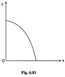
Second, since the MRS of X for Y increases as the consumer has more of X, and the MRS of Y for X increases as the consumer has more of Y along an IC, the consumer would like to have only one of the goods (either X or Y) at a time. That is, here, the consumer would have an equilibrium solution at one of the corners of his budget line.

Example 20:

Explain whether the following statements are true or false:

(i) MRS is constant at all points on an ICC.

(ii) All inferior goods are Giffen goods.

(iii) Prices of cigarettes are higher compared to those in the last year, the demand for cigarettes is also higher. Therefore, cigarettes are Giffen goods.

Solution:

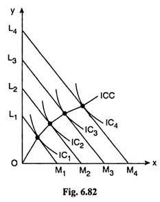
(i) The given statement is true. We may explain this in the following way by referring to Fig. 6.82.

The ICC passes through the points of tangency between the consumer’s ICs for the goods, say, X and Y, and his parallel budget lines obtained on account of successive increases in his money income, the prices of the goods remaining constant.

That is why along an ICC, the slopes of the consumer’s ICs are equal, being equal to the slope of the (parallel) budget lines and, therefore, his MRS between the goods is constant at all points on his ICC. This is because MRS_{X Y} and numerical slope of an IC at any point is itself the consumer’s MRS_{X Y}.

(ii) The given statement is not true. We may explain this in the following way: In the case of an inferior good, a rise in the consumer’s real income due to a ceteris paribus fall in the price of the good would result in a fall in the quantity purchased of the good.

This is the income effect (IE). Also, the same fall in the price of the good would make the good relatively cheaper and the consumer would purchase the good in a larger quantity. This is the substitution effect (SE)—he would substitute the relatively cheaper good for the relatively dearer good.

Now, it may very well be the case that the SE rise in the demand for the good would be greater than the IE-fall in its demand. In this case, the price effect or the total effect (i.e. IE + SE) would be that the demand for the good rises when its price falls, making the good a non-Giffen good.

Therefore, an inferior good would not necessarily be a Giffen good. It may be noted here that, by definition, the demand for a Giffen good also falls when its price falls,

(iii) In this case, the answer cannot be a straight yes or no. If the demand for cigarettes rises as their prices rise, “other things” remaining constant, then, by definition, cigarettes would be Giffen goods. Here, nothing is mentioned specifically of the “other things”.

But it is most likely that, as compared to the last year, these “other things” like the tastes and habits of the consumers, the income of the buyers, the number of buyers, etc. do not remain constant.

On the contrary, they do change giving rise to a rise in the demand for cigarettes that may surpass the fall in their demand due to a rise in their prices. In that case, although apparently cigarettes may seem to be Giffen goods, they are, actually, subject to the law of demand, i.e., they are not Giffen goods.

On the other hand, if the “other things” do remain constant or change in such a way that gives rise to a fall in the demand for cigarettes, even if their prices remain constant, then a rise in their demand as their prices rise, would certainly make cigarettes a Giffen good.

Example 21:

The utility function of an individual is U = L⁵⁷ X ⁰⁶ Y ⁰⁹ where L, X and Y stand for his weekly consumption of leisure, good X and good Y.

Assuming the rate of wage to be W per hour, calculate his utility-maximising hours of leisure and work per week, the proportion of income spent on good X, the coefficient of price- elasticity of demand for good X and income-elasticity of demand for good Y.

Solution:

The utility function of an individual is given as:

U = L⁵⁷ X⁰⁶ Y⁰⁹                                (1)

where L, X and Y stand for the quantities of weekly consumption of leisure, good X and good Y.

If the rate of wage is W per hour, then the budget constraint of the individual is

7 x 24 W = WL + P_x.X + P_Y.Y              (2)

where 7 x 24 W = his total weekly income

P_x = price of good X and

P_Y = price of good Y.

In order to obtain the conditions for utility maximisation, let us construct the relevant Lagrange function:

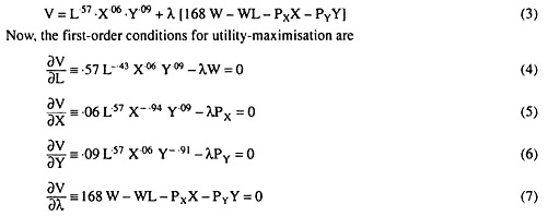
Dividing (5) by (4), after suitably transposing terms:

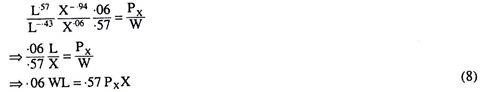
Again, from (4) and (6), we have

Adding (8) and (9):

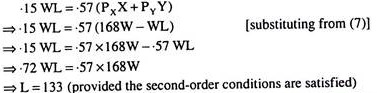
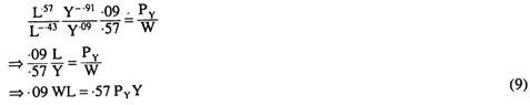
i.e., the consumer should take 133 hours of leisure in a week and, therefore, he should work (168 – 133) hours or 35 hours per week.

Putting L = 133 in (2), we have

Where 35 W is his income per week, 35 hours being his amount of work per week.

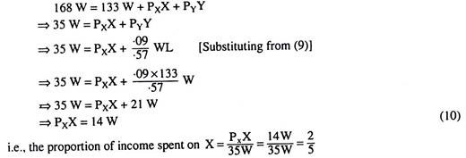
The coefficient of price-elasticity of demand for X is

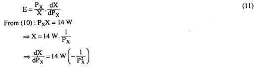
Therefore, from (11), we have the coefficient of price-elasticity of demand to be

So the numerical coefficient of price-elasticity of demand for X is e = 1

Lastly, the income elasticity of demand for Y is

where M stand for consumer’s money income. We have obtained L = 133 and M = 35 W.

So from the budget constraint (2), we have

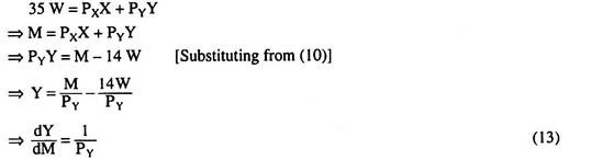
Therefore, from (12):

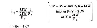
i.e., the coefficient of income elasticity of demand for Y is 1.67.

Example 22:

Suppose that the consumer spends his entire income on commodities X and Y.

On the basis of his budget constraint, show that:

(a) The expenditure-share weighted sum of the income elasticities equals unity.

(b) When X and Y are neither complements nor substitutes, then the expenditure-share weighted sum of own price-elasticities equals unity with a negative sign.

Solution:

(a) We are given that the consumer spends his entire income (M) on two goods, X (with price = p_x) and Y (with price = p_Y). That is, we have

M = p_xx + p_Yy (1)

From (1), taking total differential, we have

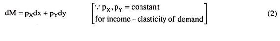
Now, by definition, the coefficient of income-elasticity of demand for goods X and Y are,, respectively,

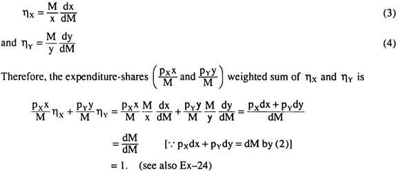
(b) The consumer’s budget constraint is

Where M = constant

Taking total differential of (5), we have

[^._.^. dM = 0 and dp_y = 0 in the case of price-elasticity of demand for X]

Multiplying (6) through by p_xxy/M_xy dpx, we obtain

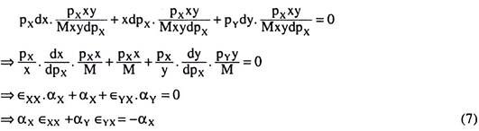
where ϵ_XX = coefficient of cross-elasticity of demand for X w.r.t. p_x

ϵ_YX = coefficient of cross-elasticity of demand for Y w.r.t. p_x

α_x = expenditure share of good X

α_Y = expenditure share of good Y Again, taking total differential of (5), we have

0 = p_xdx + p_Ydy + ydp_Y (8)

[^._.^. dM = 0 and dp_x = 0 in the case of price-elasticity of demand for Y]

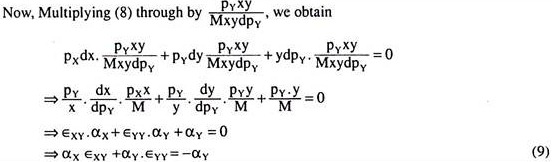
where ϵ_XY = cross-elasticity of demand for X w.r.t. p_Y

ϵ_YY = elasticity of demand for Y w.r.t. p_Y.

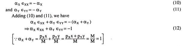
Now, since the goods X and Y are neither substitutes nor complements, we have the cross- elasticities equal to zero, i.e., ϵ_XY = 0 and ϵ_YX= 0. Therefore, from (7) and (9), we have

Example 23:

Derive the relations between own-and cross-price elasticities of demand for com­pensated demand functions.

Solution:

Let us suppose that the utility function of the consumer is

U = f(q₁,q₂)                                  (1)

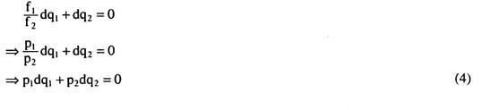
Taking the total differential of utility function (1) and letting dU = 0, we have

F₁dq₁+f₂dq₂ = 0                          (2)

As we know, the first-order condition for utility maximisation is

Where p₁ and p₂ are the prices of the goods.

Form (2) and (3), we have

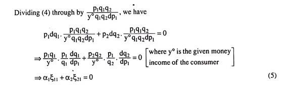
Where α₁ = expenditure-share of good Q₁

α₂ = expenditure-share of good Q₂

ξ₁₁= elasticity of demand for Q₁ w.r.t. pi for compensated demand (c. d.) function

ξ₂₁= cross-elasticity of demand for Q₂ w.r.t. p₁ for compensated demand function.

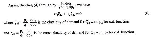
(5) and (6) give us the relations between own and cross price-elasticities of demand for compensated demand functions.

Adding (5) and (6), we obtain:

(7) gives us another relation between the own- and cross price-elasticities of demand for c.d. function. (7) gives us that the sum of the expenditure-share weighted sums of own- and cross price-elasticities of demand for the two goods for c.d. function is equal to zero.

Example 24:

Show that in a two-good model, the sum of expenditure-share weighted income- elasticities of the goods is equal to one.

Solution:

In the two-good (Q₁, Q₂) model, the budget constraint of the consumer is:

P₁q₁ + P₂q₂ = y°                                (1)

where p₁ and p₂ are the prices of the two goods.

Taking total differential of (1) w.r.t. y (p₁, p₂ = constant, in the case of income-elasticity of demand), we obtain:

P₁dq₁ + p₂dq₂ = dy                             (2)

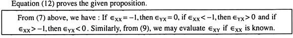
Multiplying through by y/y, multiplying the first term on the left by q₁/q₁, the second by q₂/q₂ and dividing through by dy, we have

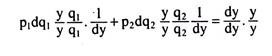
Equation (3) proves the given proposition.

Example 25:

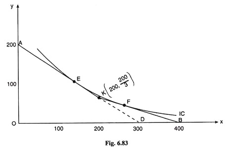
The price of good X is Rs 2 for the first 200 units and Re 1 for all units purchased in excess of 200. Good Y sells at a constant price of Rs 3.

(a) Sketch the budget set for income of Rs 600.

(b) Is it possible to have more than one equilibrium?

(c) Will the consumer ever purchase exactly 200 units of X?

Solution:

(a) The price of good Y is constant at Rs 3. Therefore, for an income of Rs 600, the y-intercept of the budget line would be 200. For the first 200 units of X, the price of X is Rs 2. Therefore, over this range (0 ≤ x ≤ 200), the numerical slope of the budget line is p_X/p_Y = 2/3and for the purchase of X in excess of 200 units, p_x = Re 1.

Therefore, for x > 200, the numerical slope of the budget line is p_X /p_Y= Also, for the first 200 units of purchase of X at p_x = Rs 2, the consumer spends Rs 400, and with the remaining Rs. 200 (= 600 – 400), the consumer would be able to purchase another 200 units at p_x = Re 1.

That is, under the given conditions, if the consumer spends all his money (Rs 600) on good X, he would be able to purchase 400 units of the good—first 200 at p_x = Rs 2 and the next 200 at p_x = Re 1. With all these specifications, we have sketched the consumer’s budget line AKB in Fig. 6.83. The line would have a kink at the point K because, here the line changes its numerical slope from 2/3 to 1/3. The coordinates of point K is (x = 200, y =200/3)

(b) It can be seen in Fig. 6.83 that with the budget line AKB, it is possible for an indifference curve, viz., IC to touch the budget line at two points like E and F. This is possible because of the kink at the point K.

(c) At x = 200 units or at the point K (200, 200/2), there is a kink. That is why, a convex-to- the-origin continuous IC cannot touch the budget line at this point. Therefore, the consumer can never be in equilibrium at the point K, i.e., he would never purchase x = 200 units in the given case.

Example 26:

Under initial prices, the consumer is purchasing 100 units of commodity X. Government then levies an additional tax of Re 1 per unit which raises the price of X by Re 1 per unit. Not wanting to hurt the consumer, Government also gives him a Rs 100 of income subsidy.

(i) Will there be any change in the level of utility of the consumer? Explain.

(ii) Will there be any change in the demand for X compared to the initial situation (before both tax and subsidy)? Explain.

Solution:

Let us answer the questions with the help of Fig. 6.84. Here we have assumed that the consumer buys the two goods X and Y. We have also assumed that, initially, the budget line of the consumer is L₁M₁ and he is in equilibrium at the point E₁ where the budget line has touched one of his indifference curves, viz., IC₁. As we are told, at E₁, the consumer buys x₁ = 100 units of good X.

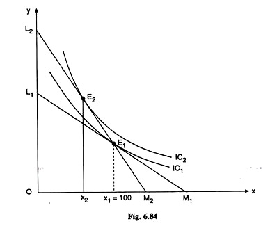
Now, as the government imposes a tax of Re 1 per unit and the price of X (p_x) increases by Re 1 per unit, the price of good Y (p_Y) remaining the same, the relative price of X increases and his budget line becomes steeper. This is because the numerical slope of the budget line is equal to the ratio of p_x and p_Y, and, here, p_x has increased.

Also, as a result of the imposition of the tax, the cost of buying x₁ = 100 units of good X increases by Rs 100, and therefore, the cost of buying the (x, y) combination, E₁ increases by the same amount. However, as the government gives the consumer an income subsidy of Rs 100, the consumer can buy the combination E₁ as before, if he so desires, even after the impo­sition of the tax.

This gives us that the post-tax and post-subsidy budget line of the consumer is steeper than his initial budget line, L₁M₁ but the new budget line would pass through the point E₁. Therefore, it would be a line like L₂M₂, and its numerical slope would be equal to the post- tax price ratio.

We are now in a position to answer question:

(i) Although E₁ is a point on the budget line L₂M₂, the consumer would no longer be in equilibrium at this point because E₁ is not a point of tangency. Rather, the consumer would be in equilibrium at the point E₂ where the budget line L₂M₂ has touched one of his ICs, viz., IC₂.

Since IC₂ is a higher curve than IC₁, the consumer’s level of utility would be higher in the post-tax, post-subsidy situation. It may be noted that the line L₂M₂ can be tangent to a higher curve only than IC₁, if the ICs are non-intersecting.

Let us now answer question:

(ii) Since the line L₂M₂ can touch one of the non-intersecting ICs at a point like E₂ that may lie only to the north-west of E₁, the consumer, in the new situation, would buy good X in a smaller quantity. The reason is obvious.

In the post-tax, post- subsidy situation, the consumer’s loss in real income has been compensated for by the subsidy (in the Slutsky sense), but since good X has become relatively dearer in the process, the substi­tution effect brings about a fall in his demand for X.