Introspective Cardinalist Theory | Microeconomics

In this article we will discuss about the introspective cardinalist theory of consumer behaviour as developed by Sir Alfred Marshall.

1. The Law of Diminishing Marginal Utility:

In Marshall’s theory, utility is cardinally measurable in terms of money. According to the Marshallian law of diminishing marginal utility (LDMU), as the consumer goes on consuming a certain good, the marginal utility derived from its consumption diminishes.

By marginal utility, means the utility derived from the consumption of the marginal (or an additional) unit of the good. More formally, MU is defined as the increment in total utility (TU) obtained as a result of consumption of one additional unit of the good. Or, MU is the rate of change of TU

w.r.t. the quantity (q) consumed of the good, i.e., MU = d/dq (TU).

It is only the consumer who, through introspection, can tell that as he goes on consuming more and more of a good, the marginal utility diminishes. The LDMU is also not unrealistic, because it is quite possible that as the consumer goes on having more and more of a good, his want is satisfied more and more and, therefore, to him the utility of the marginal unit diminishes.

the LDMU can be illustrated with the help of the following table:

Table 5.1: Total and Marginal Utility Schedule of a Consumer in the Consumption of a Particular Good

2. Total Utility and Marginal Utility Functions:

The functional relationships between the total utility (TU) derived by the consumer and the quantity consumed (q) of the good and that between the marginal utility (MU) and q have been illustrated in the columns (1) and (2) and (1) and (3) of Table 5.1. Columns (1) and (2) gives the total utility function of the consumer—total utility is a function of q.

As q increases, TU also increases, so long as MU, although diminishing, is positive. But as consumption increases beyond a certain quantity, the (diminishing) MU becomes negative and the TU starts falling.

Similarly, columns (1) and (3) gives the MU function of the consumer—MU is a function of q. As q increases MU diminishes monotonically, and, ultimately, it becomes equal to zero and then negative—this is the famous law of diminishing marginal utility.

3. TU and MU Curves:

The graphical constructions of the TU and the MU functions, which are known as TU and MU curves, for the data of Table 5.1, have been shown in Fig. 5.1.

Note the following points in these constructions:

(i) The utility obtained from the first unit of the good is Rs 10. When the consumer con­sumes only one unit, the first unit is the marginal unit and so, at q = 1, both TU and MU are equal to Rs 10 (TU = MU = Rs 10). In other words, both the TU and the MU curves start from the same point and this point is (q = 1, TU = MU = Rs 10).

(ii) As q increases, TU increases at a diminishing rate. That is why the TU curve has been obtained to be concave downwards.

(iii) At q = 11 in Fig. 5.1, the TU curve’s rise with the rise in q stops as MU becomes equal to zero. That is, TU is maximum at q = 11.

(iv) As q rises beyond q = 11, MU becomes negative and its negative magnitude rises be­cause of dMU. Therefore, now TU falls at an increasing rate.

(v) The points (ii) and (iv) give us that the TU curve would be parabolic, being concave downwards to the horizontal axis.

(vi) As q rises from q = 1, the MU curve monotonically slopes downwards towards right because of dMU. Since, in Table 5.1, the rate of fall in MU w.r.t. q is a constant, being equal to 1, the MU curve in Fig. 5.1 has been obtained to be a straight line with slope = -1.

(vii) At q = 11, MU = 0, i.e., the MU curve crosses the q-axis at q = 11, and, as q rises beyond q = 11, the MU becomes negative. As noted, at q = 11 when MU = 0, TU becomes the maximum.

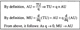
(viii) In the example of Table 5.1, q has been assumed to be a discrete variable. It assumes only, the integer values and it does not assume the fractional values. That is why TU = MU at q = 1. But if q is assumed to be a continuous variable, then TU → 0 at q →0 and marginal utility (MU) average utility (AU) as q → 0 can be obtained. (see the box below)

(ix) In our example of Table 5.1, since q is a discrete variable, TU = maximum and Rs 55 is obtained, both at q = 10 and at q = 11. But if q is a continuous variable, (TU) = 0 at q = q* where TU is maximum can be obtained, and equal to 55 (in our example), i.e., here TU = 55 in the interval dq around q = q* can be obtained, i.e., at q = q *±1/2dq where dq is infinitesimally small.

Note that, in this case, TU = 55 at q = q* = 11 and at q = q* – 1 = 10 cannot be obtained. If q* = 11 units, then it will be said that TU is maximum in the output interval 11 ± 1/2dq.

(x) In the example, q is a discrete variable. So at the discrete values of q only some discrete TU and MU points will be obtained. Of course, there will not be any difficulty in fitting a TU and an MU curve into those points, which would have obtained if q were a continuous variable.