How to Derive Indifference Curve from Revealed Preference?

This article will guide you to know about how to derive indifference curve from revealed preference.

Samuelson’s revealed preference theory has been used to derive an indifference curve in a much methodical way than the indifference curve approach. In the indifference curve technique, it is assumed that an indiffer­ence curve can be derived by asking the consumer to choose among all possible baskets or combinations of commodities.

However, consumers often cannot or will not give trustworthy answers to direct questions on their preferences. According to the theory of revealed preference, “a consumer’s preferences can be inferred and indifference curve derived from a sufficient number of observed choices or purchases in the market, without any need to inquire directly into the individual’s preferences.”

Moreover, the indifference curve technique assumes that the consumer ranks all possible combinations of commodities rationally and consist­ently. But in the revealed preference theory, the consumer is not required to rank his preferences and to give any other information about his tastes. Instead, it helps us in deriving a convex indifference curve by observing the market behaviour of the consumer.

It’s Assumptions:

This analysis is based on the following assumptions:

(1) The consumer’s tastes do not change.

(2) He prefers a combination of more goods to less in any situation.

(3) There is consistency in consumer’s behaviour. It means that if A is preferred to В in one situation, В cannot be preferred to A in the other situation

(4) There is transitivity in consumer’s preferences. It means that if A is preferred to B, and В to C, then the consumer must prefer A to C.

(5) There are two goods X and Y.

Given these assumptions, the consumer chooses a particular combination of the two goods over another for one of the two reasons: either the chosen combination is preferred to all other combinations, or the one which is not chosen lies outside his budget line.

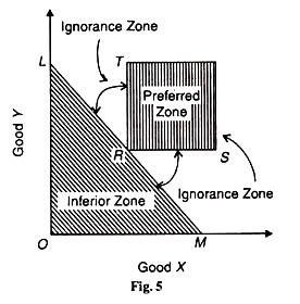
Suppose the consumer reveals his preference for combination R on his initial budget line LM in Figure 5. All other points on and below the line LM show inferior combi­nations to R. This is denoted by the shaded area and is called the inferior zone.

On the other hand, points above and/or to the right of R in the area TRS are preferred to R because they have more of X and/or Y. Thus the shaded area TRS above R is called the preferred zone. Still there are combinations of the two goods in the areas below TRS and above the line LM to the left and right of R that are not ordered by the consumer.

They are TRL and SRM and are called ignorance zones be­cause the consumer’s preferences are not known in them. It follows that the indifference curve must pass through R and lie below the area TRS and above the budget line LM. It must be negatively sloped and convex to the origin at point R, as it will be in the upper and lower zones of ignorance.

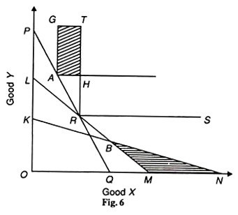
To find out the exact location of the indifference curve, let us first suppose that the price of X falls so that the consumer’s new budget line is KN which cuts the initial line LM at В below point R in Figure 6.

Now the consumer will choose either combination В or any other combination on the BN segment of the line KN. All other points on the KB segment of this line to the left of В would be inconsistent with his choice because they lie in the inferior zone below the original budget line LM.

Since the consumer chooses the combination B, it is revealed inferior to R and every point on or below the BN segment is also revealed inferior to R. Thus the triangle BNM is chopped off from the lower ignorance zone. By drawing such budget lines below point R and applying the same reasoning, the entire portion below R in the lower ignorance zone can be eliminated.

Similarly, we can chop off points to the left of R in the upper ignorance zone of Figure 6. Sup­pose the price of X increases and the new budget line PQ passes through the original point R which shows the same real income as at point R.

Consider that the consumer chooses a new point, say, A on the budget line PO. Thus he reveals his preference for A to R, both being on the same budget line. But all combinations in the area GAH to the right and above A are preferred to A because this area repre­sents combinations which have more of one of the goods than combination A.

In other words, since A is preferred R and GAH is preferred to A. therefore GAH is preferred to R. Thus by ranking the combinations in the area GAHT as preferred to R. we have eliminated some of the upper ignorance zone.

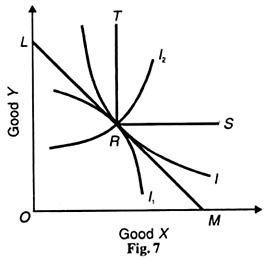
By repeating this procedure, we narrow down the ignorance zone and ultimately locate the indifference curve, shown as I in Figure 7 So far as the shape of the indifference curve is concerned Figure 7 shows the I curve to be convex to the origin at point R because it passes through the lower and upper ignorance zones.

To give further proofs, first we consider LM as the straight line indifference curve. The line LM cannot be an indifference curve because the choice of R reveals all other points on LM to be inferior to R and the consumer cannot be at the same time indifferent between point R and any other point on LM.

Second, it cannot be a curve, like I₂ in the figure, intersecting the line LM at point R because all points below R have been revealed inferior to R and the consumer is indifferent to them. Third, the indifference curve cannot be concave through R like the curve I₁ because the upper and lower portions of this curve are in the inferior zone and all points have been revealed inferior to R.

Therefore, the indifference curve can only be convex to the origin, as curve I in Figure 7.