Substitution and Income Effect (With Equations)| Consumer

In this article we will discuss about the substitution and income effect on the budget of a consumer.

Let’s assume that the ordinal utility function of the consumer is

U = f(q₁,q₂)           [eq. (6.1)]

where q₁ and q₂ are the quantities of the goods Q₁ and Q₂, respectively, and U is the ordinal utility number.

The consumer’s budget constraint can be written as y^o = p₁q₁ + p₂q₂          [eq. (6.23)]

where y^o is his income which is fixed and given, and p₁p₂ are the given prices of the two goods.

The rational consumer is to maximise U as given by (6.1) subject to the budget constraint (6.23).

In order to find out the conditions for such constrained maximisation, let’s form the relevant Lagrange function:

V = f (q₁,q₂) + λ (y° − p₁q₂ − p₂q₂)                    [eq. (6.24)]

where λ is the Lagrange multiplier and V is a function of q₁ q₂ and λ. Also V is identically equal to U for those values of q₁ and q₂ that satisfy the budget constraint. Constrained maximisation of U would then be the same thing as the simple maximisation of V.

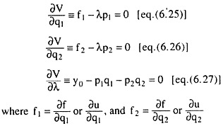
The first- order conditions (FOCs) of the constrained maximisation of U then would be given by:

 

 

 

 

 

 

 

The quantities purchased by a rational consumer would always satisfy eqns. (6.25)-(6.27). Changes in prices and income will normally alter his purchase plan, but the new quantities (and prices and income) must satisfy the conditions (6.25)-(6.27) if U is to be maximised.

Find the magnitudes of the effects of price and income changes on the consumer’s purchases. To do this, allow all the parameters, viz., p₁p₂ and y, to vary simultaneously. Also assume that as a result of these autonomous changes, the quantities purchased by the consumer would change by dq₁ and dq₂.

Taking total differentials of (6.25)-(6.27), we have:

F₁₁dq₁ + f₁₂dq₂ – p₁dλ = λ dp₁  ………..(6.64)

F₂₁dq₁ + f₂₂dq₂ – p₂dλ = λ dp₁ ……………(6.65)

−p₁dq₁ –p₂dq₂ = − dy + q₁dp₁ + q₂dp₂ ……..(6.66)

Before solving the equation system (6.64)-(6.66), let us note that the terms on the RHS of these equations are constants and they are known to us because these terms involve the autonomous changes and the initial values of different variables.

The array of coefficients on the LHSs of the equation form the following bordered Hessian determinant:

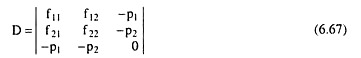
The solutions of the equation system (6.64)-(6.66) obtained with the help of Cramer’s rule, would be:

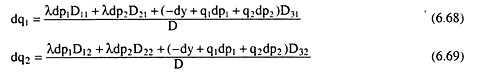
Where D_ij is the cofactor of the element in the ith row and jth column of D.

Dividing both sides of (6.68) by dp₁ and assuming that p₂ and y do not change (i.e., dp₂ = dy = 0), we have

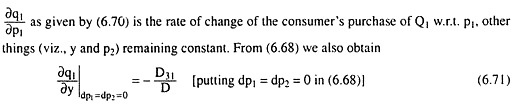
Now consider a price change that is compensated by an income change that leaves the consumer on his initial indifference curve. In this case, we would get

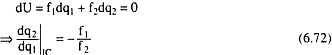
Since, in equilibrium, f₁/f₂ = p₁p₂, (6.27) gives

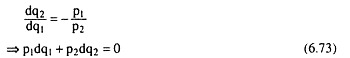
Hence from equation (6.66) we obtain

and from (6.68), we obtain

 

 

 

Therefore, (6.70) can now be written:

 

 

Equation (6.5) is known as the Slutsky equation. Now note that p₂,q₁ and q₂ remaining constant, if there is a rise (fall) in p₁ by small one unit of money, the expenditure of the consumer would also rise (fall) by ∂/∂p₁ (p₁q₁ + p₂q₂) = q₁units of money.

This rise (fall) in expenditure would compel the consumer to borrow (save) q₁ units of money to maintain his purchase plan (q₁, q₂). That is why, this rise (fall) in expenditure by q₁ units of money is equivalent of a fall (rise) in his (real) income by q₁ units of money.

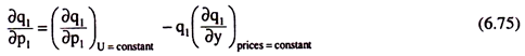
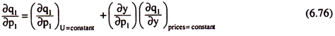
So it may be written as ∂y/∂p₁ = -q₁ (units of money) and substitute this in (6.75) to obtain the Slutsky equation in different form as given by (6.76) below:

 

 

 

 

Hicks and Slutsky Compensation Demand:

The quantity ∂q₁/∂p₁ on the L.H.S of Slutsky equation (6.75) or (6.76) is the slop of the ordinary demand function for Q₁, and the first term on the RHS is the slope of the compensated demand function for Q₁ (based on the Hicksian compensation criterion).

An alternative compensation criterion (the Slutsky criterion) is that the consumer is provided enough income to purchase his former consumption bundle so that dy = q₁dp₁ + q₂dp₂. This is

 

 

 

 

  Which can be substituted for the 1^st term on the RHS of (6.75) or (6.76).

At first sight, it might puzzle s that the two rather different compensation schemes led to the same result. However, they only refer to the same derivation, i.e., they only refer to a change in q for an infinitesimally small change n p at a point, and may lead to quite different result for any finite price movement. In other words, for an infinitesimally small change in p₁,

 

 

show quite different effect upon q₁.

Elasticity Form of the Slutsky Equation (Elasticities of Ordinary and Compensated Demand):

The Slutsky equation may also be expressed in terms of the price and income elasticities.

Multiplying (6.75) by p₁/q₁ and multiplying the last term on RHS by y/y, we get

 

 

 

 

 

 

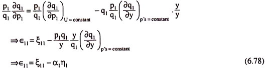
Equation (6.78) is the elasticity representation of the Slutsky equation (6.75) or (6.76). It gives that the price-elasticity of the ordinary demand curve (ϵ₁₁) equals the price-elasticity of the compensated demand curve (ξ₁₁) less the corresponding income-elasticity (η₁) due to the change in p, multiplied by the proportion of total expenditure on Q,.

Hence, the ordinary demand curve will have a smaller elasticity than the compensated demand curve, considering the negative values of ϵ₁₁ and ξ₁₁ and the positive value of r|,. That is, numerically, the ordi­nary demand curve will have a greater elasticity than the compensated demand curve.

Direct Effects:

The first term on the RHS of (6.75) or (6.76) is the substitution effect (SE) or the rate at which the consumer substitutes Q₁ for Q₂ when the price of Q₁ changes and he moves along a given IC. The second term on the right is the income effect (EE) of a change in p₁.

 

 

 

 

 

 

 

 

 

 

 

 

 

Assume now that only income changes and dp₁ = dp₂ = 0. Then (6.81) becomes

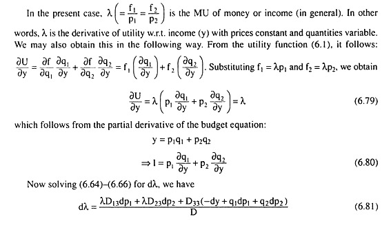
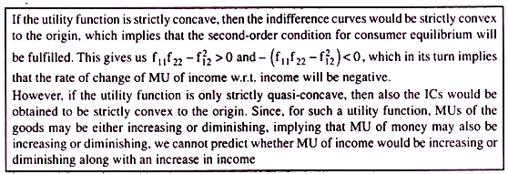
Since D is positive, the rate of change of MU of income w.r.t. income will have the same sign as -(f₁₁f₂₂^— f²₁₂). This would be negative if the utility function were strictly concave. How­ever, for ordinal utility functions, only strict quasi-concavity is assumed, and the theory does not predict whether the MU of income is increasing or decreasing with income.

By (6.74), the SE is (D₁₁/D) λ. Since D is positive, D₁₁ = −p²₂ is negative and X is positive, the SE is clearly negative. This proves that the sign of the SE is always negative and the compensated demand curve is always downward sloping.

A change in real income may cause a reallocation of consumer’s resources even if the relative prices do not change, i.e., if the absolute prices do not change or if they change in the same proportion. The income effect of a change in p₁ is (∂y/∂p₁).(∂q₁/∂y)_{p’s = const.} and it may be of either sign. The final effect of a price change on the purchase of the commodity is thus unknown.

However, an important conclusion can still be derived. The smaller the quantity of Q₁, the smaller would be the value of ∂y/∂p₁ and the less significant is the income effect. A commodity Q₁ is called an inferior good if the consumer’s purchase diminishes as income rises and in- creases as income falls, i.e., ∂q₁/∂y if is negative, and this makes the income effect positive (for ∂y/∂p₁ is always negative).

In other words, income effect for an inferior good is positive.

A Giffen good is an inferior good with a positive income effect large enough to offset the negative substitution effect and make the price effect, ∂q₁/∂p₁, positive. This means that if Q₁ is a Giffen good, then as p₁ falls, q₁ also falls.

This may occur if a consumer is sufficiently poor so that a considerable portion of his income is spent on a commodity such as wheat which he needs for his subsistence. Assume that the price of wheat falls.

The consumer who is not very fond of wheat may suddenly discover that his real income has increased substantially as a result of the price fall. He will then buy a smaller quantity of wheat and purchase a more palatable diet with the remainder of his income.

The Slutsky Equation for a Specific Function—an Illustrative Example:

The Slutsky equation can be derived for the specific utility function U = q₁q₂ (1)

The budget constraint in the general implicit form is: y₀ – p₁q₁ – p₂q₂ = 0 (2)

Form the Lagrange function V = q₁q₂ + X (y₀ – p₁q₁ – p₂q₂) (3)

Setting the partial derivatives equal to zero:

 

 

 

 

 

 

 

 

 

 

 

 

 

 

 

 

 

 

 

 

 

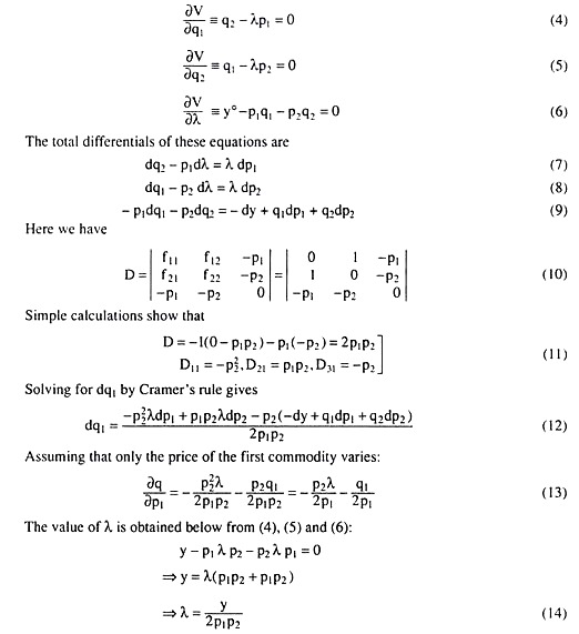
From (13) and (14):

 

 

 

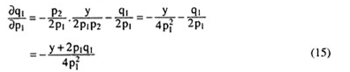
Now asume y = 100, p₁ = 2, p₂ = 5, the equilibrium values of q₁ and q₂ would be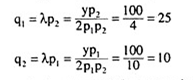

 

 

 

Now substituting the required values in (15), a numerical answer is obtained

 

 

The meaning of this answer is this. If starting from the initial equilibrium situation, p₁ were to change, ceteris paribus, the consumer’s purchase of Q₁ would change in the opposite direction at the rate of 12. Units per doller of change in the price of Q₁.

The expression –p₂λ/2p₁ in (13) is the SE, and its value in the present example is p₂λ/2p₁ = – [(p₂/2p₁)(y/2p₁p₂)] = – [(5/2×2)(100/2x2x5)] = – 6.25. The expression – q₁/2p₁ in (13) is the income effect. Its value is also – 6.25.

Cross Effects:

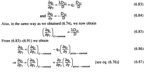
The Slutsky equation (6.75) and its elasticity form (6.78) may be extend to explain how the demand for one of the goods (Q₁) would change because of changes in the price of another good (Q₂). From (6.68), we obtain

 

 

 

 

 

 

 

 

 

 

 

 

 

 

Here ϵ₁₂ = price-elasticity of ordinary demand for Q₁ w.r.t. p₂,

ξ₁₂ = price-elasticity of compensated demand for Q₁ w.r.t. p₂,

η₁ = income-elasticity of demand for Q₁

and α₂ = proportion of total expenditures spent on Q₂.

Therefore, eqn (6.88) gives that the cross-elasticity of ordinary demand for Q₁ w.r.t. p₂ equals the cross-elasticity of compensated demand for Q₁ w.r.t. p₂ minus the income-elasticity of demand for Q₁ multiplied by the proportion of total expenditures spent on Q₂.

Now, the sign of the cross substitution effect is not known in general. Let S₁₂ = D₂₁λ/D denote the substitution effect when the quantity of Q₁ is adjusted as a result of variation in the price of Q₂. Since D is a symmetric determinant, D₁₂ = D₂₁, and it follows that S₁₂ = S₂₁.

That is, the substitution effect (SE) on Q₁ resulting from a change in p₂ is the same as the SE on Q₂ resulting from a change in p₁. This is indeed a remarkable conclusion. The sum of the compensated demand elasticities for Q₁ as a result of changes in p₁ and p₂ is

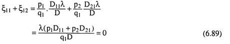
Here P₁D₁₁ + p₂D₂₁ equals zero, since it is an expansion of the determinant of (6.64)-(6.66) in terms of alien cofactors, i.e., the cofactors of the elements of the first column are multiplied by the negative of the elements in the last column. From (6.89), we have

ξ₁₁ + ξ₁₂ (6.90)

i.e., the compensated elasticity of demand for Q, w.r.t. p, is equal to the negative of the com­pensated elasticity of demand for Q, w.r.t. p₂. Now obtaining another interesting conclusion.

The sum of the negative of the ordinary demand elasticities for Q, caused by changes in p, and p₂ as given by (6.78) and (6.88) is:

Therefore, it is obtained that the income-elasticity of demand for a commodity equals the negative of the sum of ordinary price-elasticities of demand for that commodity w.r.t. its own and the other price. In other words, the sum of the own price elasticity, cross price elasticity and income-elasticity of demand for a commodity in a two-good model is equal to zero.

Substitutes and Complements:

Loosely defined, two commodities are substitutes if one of them can be used by the consumer for the other, and they are complements if they are to be used jointly in order to satisfy some particular need. For example, tea and coffee are substitutes and tea and sugar are complements.

However, a more rigorous definition of substitutability and complementarity is provided by the cross-substitution term of the Slutsky equation (6.85), viz., D₂₁λ/D. The goods Q₁ and Q₂ are substitutes if the substitution effect given by this term is positive, and they are complements if it is negative.

If Q₁ and Q₂ are substitutes, loosely speaking, and if compensating variations in income keep the consumer on the same indifference curve, an increase in the price of Q₂ will induce the consumer to substitute Q₁ for Q₂. Then (∂p₁/∂p₂) _{U = constant} would be positive, and it would be negative in the case of complements.

Now, all commodities cannot be complements for each other. Hence, only substitutability can occur in the present two-good case. This can be proved easily. Let’s multiply (6.70) by p₁, (6.71) by y, and (6.83) by p₂, and add. Then 

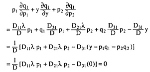
The final bracketed term is equal to zero since it is an expansion in terms of alien cofactors as in (6.89).

Therefore:

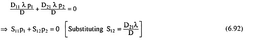
In (6.92), the substitution effect, S₁₁, for Q₁ resulting from changes in p₁ is known to be negative. Hence, (6.92) implies that S₁₂ must be positive, and this means, by definition, that Q₁ and Q₂ are necessarily substitutes.