Equilibrium of the Firm in the Short Run (With Diagram)

The firm is in equilibrium when it maximizes its profits (11), defined as the difference between total cost and total revenue:

Π = TR – TC

Given that the normal rate of profit is included in the cost items of the firm, Π is the profit above the normal rate of return on capital and the remuneration for the risk- bearing function of the entrepreneur.

The firm is in equilibrium when it produces the output that maximizes the difference between total receipts and total costs.

The equi­librium of the firm may be shown graphically in two ways. Either by using the TR and TC curves, or the MR and MC curves.

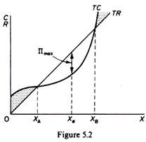
In figure 5.2 we show the total revenue and total cost curves of a firm in a perfectly competitive market. The total-revenue curve is a straight line through the origin, showing that the price is constant at all levels of output. The firm is a price-taker and can sell any amount of output at the going market price, with its TR increasing pro­portionately with its sales. The slope of the TR curve is the marginal revenue. It is constant and equal to the prevailing market price, since all units are sold at the same price. Thus in pure competition MR = AR = P.

The shape of the total-cost curve reflects the U shape of the average-cost curve, that is, the law of variable proportions. The firm maximizes its profit at the output X_e, where the distance between the TR and TC curves is the greatest. At lower and higher levels of output total profit is not maximized at levels smaller than X_A and larger than X_B the firm has losses.

The total-revenue-total-cost approach is awkward to use when firms are combined together in the study of the industry. The alternative approach, which is based on marginal cost and marginal revenue, uses price as an explicit variable, and shows clearly the behavioural rule that leads to profit maximization.

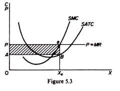
In figure 5.3 we show the average- and marginal-cost curves of the firm together with its demand curve. We said that the demand curve is also the average revenue curve and the marginal revenue curve of the firm in a perfectly competitive market. The marginal cost cuts the SATC at its minimum point. Both curves are U-shaped, reflecting the law of variable proportions which is operative in the short run during which the plant is constant. The firm is in equilibrium (maximizes its profit) at the level of output defined by the intersection of the MC and the MR curves (point e in figure 5.3).

To the left of e profit has not reached its maximum level because each unit of output to the left of X_e brings to the firm a revenue which is greater than its marginal cost. To the right of X_e each additional unit of output costs more than the revenue earned by its sale, so that a loss is made and total profit is reduced.

In summary:

(a) If MC < MR total profit has not been maximized and it pays the firm to expand its output.

(b) If MC > MR the level of total profit is being reduced and it pays the firm to cut its production.

(c) If MC = MR short-run profits are maximized.

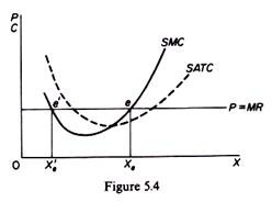
Thus the first condition for the equilibrium of the firm is that marginal cost be equal to marginal revenue. However, this condition is not sufficient, since it may be fulfilled and yet the firm may not be in equilibrium. In figure 5.4 we observe that the condition MC = MR is satisfied at point e’, yet clearly the firm is not in equilibrium, since profit is maximized at X_e > X_e^,. The second condition for equilibrium requires that the MC be rising at the point of its intersection with the MR curve.

This means that the MC must cut the MR curve from below, i.e. the slope of the MC must be steeper than the slope of the MR curve. In figure 5.4 the slope of MC is positive at e, while the slope of the MR curve is zero at all levels of output. Thus at e both conditions for equilibrium are satisfied

(i) MC = MR and

(ii) (Slope of MC) > (slope of MR).

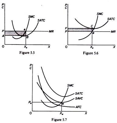
It should be noted that the MC is always positive, because the firm must spend some money in order to produce an additional unit of output. Thus at equilibrium the MR is also positive. The fact that a firm is in (short-run) equilibrium does not necessarily mean that it makes excess profits. Whether the firm makes excess profits or losses depends on the level of the, 4TC at the short-run equilibrium. If the A TC is below the price at equilibrium (figure 5.5) the firm earns excess profits (equal to the area PABe). If, however, the ATC is above the price (figure 5.6) the firm makes a loss (equal to the area FPeC).

In the latter case the firm will continue to produce only if it covers its variable costs. Otherwise it will close down, since by discontinuing its operations the firm is better off it minimizes its losses. The point at which the firm covers its variable costs is called ‘the closing-down point.’ In figure 5.7 the closing-down point of the firm is denoted by point w. If price falls below P_w the firm does not cover its variable costs and is better off if it closes down.

Mathematical derivation of the equilibrium of the firm

The firm aims at the maximization of its profit

Π = R – C

Where Π = profit

R – total revenue

C = total cost

Clearly R = ƒ₁(X) and C = ƒ₂(X), given the price P.

(a) The first-order condition for the maximization of a function is that its first derivative (with respect to X in our case) be equal to zero. Differentiating the total-profit function and equating to zero we obtain

The term ∂R/∂X is the slope of the total revenue curve, that is, the marginal revenue. The term ∂C/∂X is the slope of the total cost curve, or the marginal cost. Thus the first-order condition for profit maximization is

MR = MC

Given that MC > 0, MR must also be positive at equilibrium. Since MR = P the first-order condition may be written as MC = P.

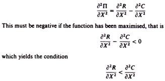
(b) The second-order condition for a maximum requires that the second derivative of the function be negative (implying that after its highest point the curve turns downwards). The second derivative of the total-profit function is

But ∂²R/∂X² is the slope of the MR curve and ∂²C/∂X² is the slope of the MC curve. Hence the second-order condition may verbally be written as follows

(slope of MR) < (slope of MC)

Thus the MC must have a steeper slope than the MR curve or the MC must cut the MR curve from below. In pure competition the slope of the MR curve is zero, hence the second-order condition is simplified as follows

0 < ∂²C/ ∂X²

Which reads the MC curve must have a positive slope, or the MC must be rising.