
In this article we will discuss about the conditions for profit maximising equilibrium of a firm.
The goal of the firm is to maximise profit. Therefore, the firm would be in equilibrium only when it achieves profit maximisation. The total revenue (TR) function of the firm gives its total revenue as a function of the quantity of output sold (q), i.e., TR = TR(q).
The total cost (TC) function of the firm, on the other hand, gives us total cost as a function of the quantity of output produced (q), i.e., TC = TC(q).
It may be noted here that the quantity of output sold per period is assumed to be the same as the quantity of output produced per period, and both are denoted by q.
ADVERTISEMENTS:
Now, profit (n) is defined to be:
π = TR(q) – TC(q) = π(q) (10.1)
Since K here is a function of q, it has to be maximised w.r.t. q.
1. The First Order Condition (FOC):
ADVERTISEMENTS:
We obtain from differential calculus that the first order or the necessary condition for profit maximisation is:
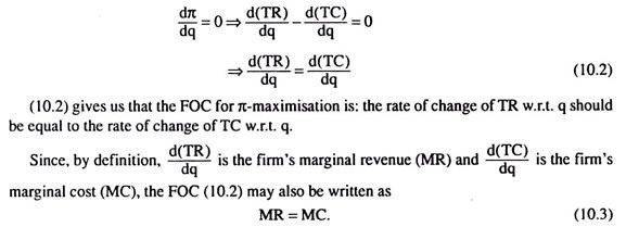
That is, if the firm is to obtain maximum profit, it would have to equate its MR and MC, or, it would have to remain at the point of intersection between its MR and MC curves.
ADVERTISEMENTS:
2. The Second Order Condition (SOC):
The first order or the necessary condition for maximum profit that we have obtained above [(10.2)] or (10.3)] is also the first order or the necessary condition for minimum profit. That is why there should be an additional condition that should be satisfied along with the FOC. This condition is called the second order condition (SOC) or the sufficient condition for profit maximisation. From calculus, we obtain the SOC as
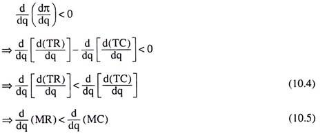
Eqns (10.4) and (10.5) are two different forms of the SOC. (10.4) gives us that the firm’s profit would be maximum if, at the point where the FOC is satisfied (i.e., at the MR = MC point), the rate of change of the slope of the TR curve is less than the rate of change of the slope of the TC curve; and (10.5) gives us that, at the MR = MC point, or, at the point of equality of the slopes of the TR and TC curves, the rate of change of MR, or, the slope of the MR curve, should be less than the rate of change of MC, or, the slope of the MC curve.
Total Revenue, Total Cost and Maximum Profit:
Perfectly Competitive Market:
We may now explain diagrammatically the FOC and SOC given by (10.2) and (10.4), respectively, for the firm’s maximum profit equilibrium. In Fig. 10.1, it has been assumed that there is perfect competition in the market for the good the firm produces and sells, i.e., it can sell any quantity at the given market price.
That is why, in Fig. 10.1, the total revenue (TR) curve of the firm has been a straight line from the origin and sloping upward towards right. In this figure, the firm’s short-run total cost curve is TC. Here N0 is the break-even (BE) point of the firm and qBE its break-even output, i.e., at the point N0, or, at q = qBE, firm’s total revenue and total cost have broken even or have become equal.
ADVERTISEMENTS:
Owing to shapes of the TR and TC curves, the firm’s profit (π = TR – TC) would be positive at q > qBE and negative at q < qBE. Here the firm’s positive profit would be maximum at that q for which the slope of the TR curve would be equal to that of the TC curve [FOC (10.2)].
In Fig 10.1, we see that at q = q) the slope of the firm’s TC curve has been equal to the constant slope of the straight line TR curve, for, at q = q], or at the point N1 on the TC curve, the tangent to the TC curve (viz., t1) has been parallel to the TR curve. Therefore, at q = q1, the FOC (10.2) for maximum profit has been satisfied. At this q, the SOC (10.4) for maximum profit has also been satisfied.
Since the firm’s TC curve has been convex downwards at the point Nb the rate of change of the slope of TC curve has been positive at q = q1; while the rate of change of the slope of the TR curve is zero, since the TR curve is a straight line.
That is, at q = qi the rate of change of the slope of TR has been less than that of the slope of the TC, or, the SOC (10.4) for maximum profit has been satisfied. Therefore, at q = q1, the firm’s profit would be maximum and the amount of this maximum profit is M1N1.
ADVERTISEMENTS:
On the other hand, in Fig. 10.1, the firm’s profit would be negative, i.e., it would suffer a loss, at q < qBE, for now TR would be less than TC. However, at q = q2 < qBE, the slope of the TC curve has been equal to the slope of the TR curve. For the tangent t2 to the TC curve at the point N2 has been parallel to the straight line TR curve. That is, at q = q2, the FOC for a maximum or a minimum profit has been satisfied.
But, at q = q2, or, at the point N2 on the TC curve, the curve is concave downwards. So here the rate of change of the slope of the TC curve is negative, whereas, the rate of change of the slope of the TR curve is zero, since TR curve is a straight line.
Therefore, at q = q2, the rate of change of the slope of the TR curve has been greater than that of the slope of the TC curve, and so, the SOC for maximum profit has not been satisfied, rather, the SOC for the minimum profit has been satisfied. That is, at q = q2, the firm’s profit will be minimum. Here, the (minimum) profit of the firm will be – M2N2, or, the (maximum) amount of loss will be M2N2.

ADVERTISEMENTS:
Imperfectly Competitive Market:
In Fig. 10.2, it has been assumed that competition in the market for the firm’s product is not perfect. Here the market is either imperfectly competitive or monopolistic. In such a market, the firm has to decrease the price of its product if it intends to sell more per period. That is why the firm’s TR curve here would be a second degree curve like the one shown in Fig. 10.2.

In this figure, the firm’s short-run total cost (STC) curve would be TC. Here the firm’s break-even output is q = qBE. Now, at q = q, in the range q > qBE, the tangents to the TR and TC curves, viz., t1 and t2, have been parallel to each other and the slopes of the TR and TC curves have been equal, i.e., the first-order condition (10.2) for maximum profit has been satisfied.
Again, at q = q1, since the TR curve is concave downwards and the TC curve here is convex downwards, the rate of change of the slope of the TR curve has been negative, and the rate of change of the slope of the TC curve has been positive.
That is, at q = q1, the (negative) rate of change of the slope of the TR curve has been smaller than the (positive) rate of change of the slope of the TC curve. Therefore, here the SOC (10.4) for maximum profit has been satisfied.
ADVERTISEMENTS:
On the other hand, at q = q2 in the range of negative profit (i.e. q < qBE), the slopes of the TR and TC curves have been equal, since the tangents to these curves at q = q2 (not shown in the diagram) are parallel to each other. Therefore, here the FOC for maximum and minimum profit has been satisfied. However, at q = q1 both the TR and TC curves are concave downwards, the TC curve being more concave than the TR curve.
Therefore, the rates of change of the slopes of both the TC and TR curves are negative, the magnitude of the former being larger than that of the latter. Therefore, at q = q2, the rate of change of the TC curve is smaller than that of the TR curve which gives us that the SOC (10.6) for minimum (not maximum) profit is satisfied at q = q2.
Therefore, at q = q2, the firm’s profit would be minimum being equal to – N2M2 in Fig. 10.2. It may be noted here that at q = q2, the magnitude of the firm’s negative profit, i.e., the firm’s loss, is maximum.
Marginal Revenue (MR), Marginal Cost (MC) and Maximum Profit:
Perfectly Competitive Market:
ADVERTISEMENTS:
We have explained the condition for the firm’s maximum profit in terms of TR and TC. Now we shall explain the conditions (10.3) and (10.5) of maximum profit with the help of the firm’s MR and MC curves shown in Fig. 10.3. Here the MR and the MC curves are, respectively, the firm’s marginal revenue and short-run marginal cost curves.
We have assumed here that there is perfect competition in the market for the firm’s product. That is why its MR curve has been a horizontal straight line at the level of the price of its product that has been determined in the market (10.5.9). We have named this curve (or line) MR = AR, because in a perfectly competitive market with price (p) exogenously given to the firm, we obtain, at any q,
p = AR = MR (10.8)
In Fig. 10.3, the MR and MC curves have intersected at the point H1, or, at q = q1. Therefore, here the FOC (10.3) for maximum profit has been satisfied. By virtue of eqn. (10.8), the FOC for maximum profit may be written as
p = AR = MR = MC =>p = MC (10.9)
Also, at H1, the slope of the horizontal MR curve is zero and that of the upward sloping MC curve is positive. Since zero is less than positive, the second order condition (10.5) for maximum profit has also been satisfied at q = q1. Therefore, q = q1, is the firm’s profit-maximising or equilibrium output.
ADVERTISEMENTS:
We have to remember here that, since the MR curve of a competitive firm is a horizontal straight line, the slope of the MR curve at any q = 0. Therefore, under competition, the SOC for maximum profit (10.5) may also be written as
the slope of the MC curve > 0 (10.10)
Eqn. (10.10) gives us that, according to the SOC for maximum profit under perfect competition, the firm’s MC curve should be upward sloping towards right at the MR = MC point (where the FOC for maximum profit has been satisfied).
On the other hand, the firm’s MR and MC curves have also intersected at the point H2, and, so, at this point the FOC for both maximum and minimum profit has been satisfied.
But at H2, or, at q = q2, since the slope of the MR curve which is zero is greater than that of the MC curve which is negative, the SOC (10.7) for the minimum (and not (10.5) for the maximum) profit has been satisfied. Therefore, if the firm sells an output quantity of q = q2, its profit would be minimum, not maximum.


Imperfectly Competitive Market:
Lastly, let us explain the profit-maximising conditions in terms of MR and MC when the firm sells its output in an imperfectly competitive or in a monopolistic market. In Fig. 10.4, like Fig. 10.3, the MC curve is the firm’s short-run marginal cost curve. Since the firm has to reduce the price of its product if it wants to sell more per period in such a market—the firm’s AR and MR curves, both would be sloping downward towards right.
At the point of intersection H1 between the MR and MC curves, or at q = q1, in Fig. 10.4, the FOC for maximum output, MR = MC, has been satisfied. Also, at H1 the negative slope of the MR curve is less than the positive slope of the MC curve. So, here, the SOC for maximum profit has also been satisfied, In other words, the firm’s profit-maximising equilibrium output is q = q1.
However, at the point H2, or at q = q2 also, the firm’s MR and MC curves have intersected, i.e., MR has been equal to MC, i.e., the FOC for maximum or for minimum profit (10.3) has been satisfied. But, here, the firm’s MR and MC curves are both negatively sloped, and the MC curve cuts the MR curve from above, i.e., the MC curve is more steep.
Therefore, the magnitude of the slope of the MC curve has been greater than that of the MR curve. In other words, here the slope of the MC curve is smaller than that of the MR curve. Therefore, at q = q2 the SOC for minimum profit (10.7), and not that for the maximum profit (10.5) has been satisfied. In other words, at the MR = MC output, q = q2, the firm’s profit is not maximised.