The Production Possibility Curve | Trade Equilibrium | Economics

A production possibility curve is the locus of such combinations of two commodities that a country can produce, given the techniques of production and the fullest utilization of all the available factors of production. It is also called as production frontier, transformation curve, product substitution curve or an opportunity cost curve. If all the available productive resources are employed in the production of commodity X, there can be maximum possible production of this commodity with no output of the other commodity Y.

On the opposite, if all the resources are utilised in the production of Y, the country will be able to produce some maximum quantity of Y commodity with no output of X commodity. Between these two extreme situations, there can be various production possibilities involving more or less quantities of the two commodities. If production of X is to be increased, there will be diversion of resources from the production of Y to the production of X, resulting in a reduced production of Y.

The curve drawn on the basis of alternative production possibilities is called as the production possibility curve. It is based on the concept of opportunity cost. In order to produce more units of X, some units of Y have to be sacrificed. So the quantity of Y that is given up is the opportunity cost of producing a given quantity of X-commodity. That is why it is known as the opportunity cost curve.

The production possibility curve shows the maximum possible quantities of two commodities that a country can produce with the given techniques and the most efficient and fullest utilization of the productive resources. The country does not possess the capacity beyond the limit specified by the production possibility curve or the opportunity cost curve. It represents the production frontier of the country.

The output more than the production frontier is impossible. If the output of the two or one of the two commodities is below the production frontier, that indicates the unemployment or excess capacity. When the production of Y commodity is reduced to produce more units of X commodity, it signifies that Y has been transformed into X-commodity. That is the reason why the opportunity cost curve is called as the transformation curve or product substitution curve.

The slope of the opportunity cost curve is measured by the Marginal Rate of Transformation of Y into X (MRT). It is ratio of a change in the quantity of commodity Y to a change in the quantity of X commodity.

MRT_xy = δy/δx

Since additional production of X involves reduced output of Y, the MRT is negative. It signifies that the production possibility curve or opportunity cost curve slopes negatively, or it slopes downwards from left to right.

The MRT_xy can be expressed also as a ratio of the marginal cost of X to the marginal cost of Y.

It can be determined as below:

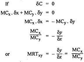
δC = MC_X. δx + MC_y. δy

Where δC = Change in cost, δx = Change in the quantity of X commodity, δy = Change in the quantity of Y commodity. MC and MC are the marginal costs of X and Y commodities respectively.

If the production is governed by constant returns, the MC_X relative to MC_y remains unchanged or MRT_xy remains the same. It means the slope of the production possibility curve or opportunity cost curve is the same and it is a negatively sloping straight line. If the production is governed by diminishing returns, MC_X rises relative to the MC_X.

It signifies that the slope or MRT_xy increases. In such a situation, the opportunity cost curve is a negatively sloping concave curve to the origin. If the production is governed by increasing returns, the MC_X decreases relative to the MC_y. The slope or MRT_xy decreases. In this case the opportunity cost curve is a negatively sloping convex curve to the origin. These cases are depicted through Fig. 4.1 (a), 4.1 (b) and 4.1(c) respectively.

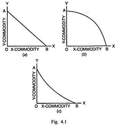
In Fig. 4.1, AB is the production possibility curve or the opportunity cost curve. In Fig. 4.1 (a), the opportunity cost curve AB is the negatively sloping straight line. Along this curve, MRT_xy= -δy/δx = MCx/MCy remains unchanged due to constant opportunity cost conditions (constant return in Fig. 4.1 (b), the opportunity cost curve AB is a negatively concave. Along it, MRTxy = -δy/δx = MC_x/MC_y increasing opportunity cost condition (diminishing returns). If Fig. 4.1 (c), the opportunity cost curves AB is a negatively sloping convex curve to the origin on account of decreasing opportunity cost condition (increasing returns).

The opportunity cost curve simply indicates the alternative production possibilities. It does not show what combinations of the two commodities will actually be produced. Haberler has employed the tool of opportunity cost curve or production possibility curve for analysing the classical trade theory in terms of the opportunity costs.