
In Fig. 11.4 and Fig. 11.5, the relative positions of the revenue and cost curves of the monopolist are such that it is possible for the firm to earn more than normal profit or pure profit.


With the help of Figs. 11.6 and 11.7, we shall now see, that these curves may be so placed that the monopolist can earn at best only the normal profit or even less than normal profit.
ADVERTISEMENTS:
In Fig. 11.6(a), the TR and TC curves of the monopolist are tangent to each other at the point E or at the output q0. Therefore, at this output the slope of the TR curve (or, the firm’s MR) is equal to the slope of the TC curve (or, the firm’s MC), i.e., the first order condition (FOC) for maximum profit has been satisfied.
Also, since the TR curve is concave downwards and the TC curve is convex downwards at the point E, the rate of change of the slope of the TR curve (which is negative) is less than that of the TC curve (which is positive) i.e., the second order condition (SOC) for the maximum profit has also been satisfied at this point.
Therefore, at the point E in Fig. 11.6(a), profit is maximised. But here, since TR = TC, the maximum amount of pure (or excess) profit is: TR – TC = 0. Here the firm is able to earn only the normal profit at best, since TR is equal to TC which includes also the normal profit.
ADVERTISEMENTS:
Here also, we may illustrate the profit-maximising equilibrium of the same firm in terms of MR and MC, and we may do this with the help of Fig. 11.6(b).
In Fig. 11.6(b), the firm is in equilibrium at q = q0 at the (MR = MC) point G. That the firm is earning only normal profit at q = q0 is obvious from the fact that here, at this output, the AR and AC curves have touched each other, and here we have AR = AC.
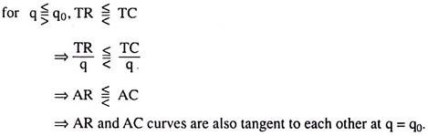
It may be noted here that if the TR and TC curves of a firm touch each other at some output, then, at the same output, the AR and AC curves of the firm would also touch each other. This we may prove in the following way.


In Fig. 11.6 (a), the TR and TC curves have been tangent to each other at q = q0, and so we obtain
Let us now come to Fig. 11.7. This figure illustrates the case where the monopoly firm earns less than the normal profit. In Fig. 11.7(a), we see that the TR curve lies below the TC curve throughout its length. In other words, whatever may be the quantity of output, the firm cannot escape incurring some amount of loss.
Here, the magnitude of negative profit or the amount of loss (= TC – TR) is minimum (= FE), i.e., profit (negative = – FE) is maximum at q=q1. At this output, the slope of the TR curve is equal to that of the TC curve (i.e., the FOC for maximum profit is fulfilled), and the rate of change of the slope of TR curve is less than that of TC curve (i.e., the SOC for maximum profit is satisfied).
The same picture is obtained also in Fig. 11.7(b). Here at q = q1, we have MR = MC (i.e., the FOC for maximum profit is fulfilled), and the slope of MR < slope of MC (i.e., the SOC for maximum profit is fulfilled).
But at q = q1 in Fig. 11.7(b), we obtain. AR < AC => AR x q1 < AC x q1 => TR < TC, which implies that, at maximum, the profit is negative. Actually, in Fig. 11.7(b), the AR curve lies below the AC curve throughout its length. This implies that whatever q may be, the firm cannot escape loss as is the case in Fig. 11.7(a) also.
It may be noted here that at q = the firm’s profit at maximum is negative. But the firm would continue production, i.e., it would not shut down, if AC > AR ≥ AVC => TC > TR ≥ TVC. For, then it would be able to use the TR – TVC surplus to pay a part of the TFC. In Fig. 11.7(b), at q = q1, we have AC > AR > AVC. So here the firm would continue production.
Its output would be q1per period. If, on the other hand, at the profit maximising or loss minimising output the firm has AC > AVC > AR => TC > TVC > TR, then it would shut down. Because, by doing this, it would be able to reduce both TVC and TR to zero and, thereby, it can save the TVC – TR portion of its loss. In this case, its loss would be equal to TC – TR = TFC + TVC – TR = TFC (TVC = 0, TR = 0).