Monopoly Equilibrium and Elasticity of Demand | Microeconomics

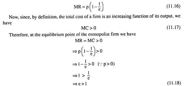
Let us now establish the proposition that monopoly equilibrium will occur at a point where the demand for the product is relatively elastic.The proposition may be established easily with the help of the relation between AR (≡ p), MR and e (e is the numerical coefficient of price-elasticity of demand). This relation is

 

 

 

 

 

 

 

 

 

 

 

which implies that the demand for the product is relatively elastic. We may now try to understand the economic significance of the above proposition with the help of Fig. 11.8. Here we have assumed, for the sake of simplicity that the AR curve or the demand curve of the firm is a negatively sloped straight line AB and, therefore, the correspond­ing marginal revenue curve is also a straight line which is the line ACD.

In Fig. 11.8, the mid­point of the line segment AB is R and, at that point, as we know, e = 1. We also know that at any point on AB below the point R, e < 1 and at any point above R, e > 1. Now, the firm cannot be in equilibrium at any point like R’ on the segment RB, where e < 1, because here, if the firm increases p, its TR would also rise. But, as p rises and q falls, its TC would fall since TC is a rising function of q.

As a result, as p rises, the firm’s profit would also rise. Therefore, at any point like R’ on the demand curve, the profit-maximising firm would increase the price of its product and move upward towards left along its demand curve. So the firm cannot be in equilibrium at a point on its demand curve where e < 1.

Next, if the firm is at the point R where e = 1, it would still like to increase the price of its product. Because, if it raises P, TR would remain unchanged, but q would fall and the TC would fall, resulting in a rise in its profit. There­fore, the firm cannot be in equilibrium at the point R where e =1.

From the above discussion, it is clear that so long as the firm is at a point on its demand curve where e ≤ 1, it would find it profitable to increase the price of its product and move upward towards left along the demand curve. But when, at the point R, it moves upward towards left along the demand curve, it finds itself on the segment AR of the demand curve, AB, where at each point e > 1.

Now, at any point with e > 1, if p rises, TR would fall and, as q falls, owing to the rise in p, TC would fall. In this case, the firm would be increasing p if, on the margin, the fall in TC is larger than the fall in TR resulting in a higher level of profit, i.e., it would raise p if MC > MR.

Now over the portion RM of the segment AR on the demand curve [or, over the output interval (q₀, OC)] in Fig. 11.8, we find MC > MR, and so the firm would be raising p till it reaches the point M at q = q₀, where MR = MC.

Again, at any point on the segment AM (with e > 1) of the demand curve, as p falls and q rises, both TR and TC would rise, and the rise in TR would be greater than the rise in TC on the margin, since here we have MR > MC, i.e., here, as p falls and q rises, the firm’s profit would rise.

So, the firm would be decreasing the price of its product along this segment (AM) till it reaches the point M where MR = MC. In other words, the monopoly firm would be in equilibrium at a point on its demand curve where e > 1 and where MR = MC. It cannot be in profit-maximising equilibrium at any point where e < 1.