
In this article we will discuss about the profit-maximising output of a monopolist firm.
The goal of a monopolistic firm is to maximise profit. Therefore, the firm would be in equilibrium when it maximises its profit. The profit (π)-function of the monopolist is
π = R(q)-C(q) = π(q) (11.12)
where π = profit, R = the firm’s total revenue (TR), and C = total cost (TC), and q = the quantity of output produced and sold by the firm.
ADVERTISEMENTS:
Now the first order condition for π-maximum is
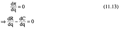
We obtain from (11.14) that the first order or necessary condition for π-maximum of a monopolist firm states that the rate of change of TR w.r.t. q, or marginal revenue (MR), should be equal to the rate of change of TC w.r.t. q, or marginal cost (MC).
ADVERTISEMENTS:
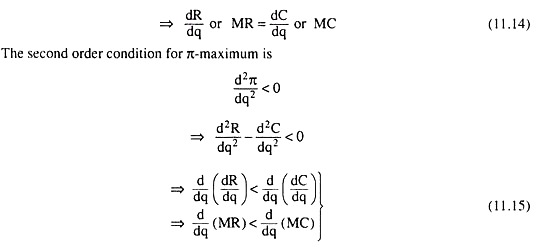
And we obtain from (11.15) that the second order or the sufficient condition for π-maximum states that the rate of change of the slope of the TR curve w.r.t. q should be less than the rate of change of the slope of the TC curve w.r.t. q, i.e., the rate of change of MR w.r.t. q should be less than the rate of change of MC w.r.t. q., i.e., the slope of the MR curve should be less than the slope of the MC curve.
The determination of the profit-maximising output of a monopolist firm may be illustrated with the help of Figs. 11.4 and 11.5. In Fig. 11.4, the profit-maximising output is q**. At this output, the slope of the TR curve has been equal to that of the TC curve as the tangents at the points E and F have been parallel. Therefore, at this output (q**), the TR – TC gap (TR > TC) is maximum.


This output satisfies the first order condition (FOC) for profit-maximisation as given by (11.14). This output also satisfies the second-order condition (11.15) since at q = q**, the TR curve is concave downwards (at point E) and the TC curve is convex downwards (at point F), i.e., at q = q**, the rate of change of the slope of the TR curve is less than that of the slope of TC curve, the former being negative and the latter positive.
ADVERTISEMENTS:
Therefore, at q = q**, the profit of the firm is maximum and the amount of this maximum profit is
π = TR-TC = EF
Incidentally, we may point out that at q = q*, the slope of the TR curve, is equal to the slope of the TC curve, i.e., the FOC (11.14) is satisfied at this output. But at this output the (TC – TR)-gap is maximum, i.e., here the profit is negative, and the loss is positive—the loss is maximum and the profit is minimum. We should remember that condition (11.14) is the FOC for both maximum and minimum profit.
However, at q = q*, the SOC (11.15) for maximum profit has not been satisfied, since here both the TR and TC curves are concave downwards and the concavity of the TC curve is larger than that of the TR curve. That is why, here, the rates of change of the slopes of both TR and TC curves are negative, but the former is larger than the latter, and so, the SOC is not satisfied at q = q*.
We may also illustrate the profit-maximising equilibrium of the same monopoly firm in terms of MR and MC. Since the TR curve in Fig. 11.4 is a second degree curve, the AR and MR curves of the firm would be of first degree, i.e., they would be straight lines, and it follows from the concave downwards shape of the TR curve that the AR and MR curves would be negatively sloped straight lines, like the ones shown in Fig. 11.5. On the other hand, it follows from the third degree shape of the TC curve that the AC and MC curves of the firm would be U-shaped like the curves shown in Fig. 11.5.
Now at q = q**, the slopes of the TR and TC curves have been equal in Fig. 11.4 which gives us MR = MC in Fig. 11.5, i.e., at q = q**, the FOC for maximum profit has been satisfied in terms of MR and MC. Also, at q = q**, the TR curve is concave downwards (at the point E) and the TC curve is convex downwards (at the point F), in Fig. 11.4.
That is why at the same output in Fig. 11.5, the rate of change of MR or the slope of the MR curve has been less than the rate of change of MC, or, the slope of the MC curve, the former being negative and the latter positive.
Therefore, the SOC for profit maximisation is also satisfied, in terms of MR and MC. In Fig. 11.5, the negatively sloped MR curve and the positively sloped MC curve have intersected at the profit-maximising point G.
ADVERTISEMENTS:
Incidentally, it may be pointed out that at q = q*, the slopes of the TR and TC curves being equal in Fig. 11.4, we have MR = MC in Fig. 11.5. That is, at q = q*, the FOC for maximum profit, which is also the FOC for minimum profit, is satisfied.
However, at q = q*, the SOC for minimum profit rather than that for the maximum profit, has been satisfied. For, at q = q*, both the TR and TC curves in Fig. 11.4 are concave downwards and the latter is more concave than the former.
This gives us that, at q = q*, the slope of the MC curve is smaller than that of the MR curve. Therefore, at q = q* in Fig. 11.5, the SOC for minimum profit, rather than that for the maximum profit, has been satisfied.
We have seen above how the profit-maximising output of the monopolist is determined on the basis of the first order and second order conditions for maximum. Once the output-quantity is determined, the firm can know from its AR curve what price it would have to charge for selling this quantity.
ADVERTISEMENTS:
For example, in Fig. 11.5, we see that the π-max quantity q = q** can be sold if the firm charges the price p = p**. In Fig. 11.5, it is seen that at q = q**, p or AR exceeds AC (average cost) by MN. So at q = q**, the average amount of profit per unit of output is
AR – AC = MN, and the total amount of profit is π = q** x MN = Dp** MNS. This is the maximum possible amount of economic profit (in excess of normal profit, since normal profit is assumed to be included in cost of production) that the firm can earn subject to its revenue and cost curves.
We may now make the following observations in respect of profit-maximising behaviour of the firm:
(i) So long as MR > MC, the firm’s profit on the margin (or its marginal profit = MR – MC) is positive, and so the profit-maximising firm would go on increasing its q till MR becomes equal to MC (i.e., the first order condition for π-max is satisfied).
ADVERTISEMENTS:
The firm would not proceed beyond the MR = MC point if, as q rises, MC becomes larger than MR, i.e., the slope of the MC becomes larger than that of the MR (i.e., the 2nd order condition for π-max is satisfied). Such an MR = MC point is the profit-maximising point G in Fig. 11.5.
(ii) If at an MR = MC point like H in Fig. 11.5, MC becomes smaller than MR as q rises, then the firm would proceed beyond that MR = MC point or beyond the output of q*, because, now, the profit on the margin is positive.
This can happen if, at the MR = MC point, the slope of the MR curve is greater than that of the MC curve, i.e., if the SOC for profit-maximisation is not satisfied, rather, the SOC for the minimum profit is satisfied. This has happened at point H.
It may be noted that at each output less than q* in Fig. 11.5, MR is less than MC, i.e., the profit on the margin is always negative for q < q*. So at q = q*, the total profit is negative maximum, i.e., here the (positive) profit is minimum and the (positive) loss is maximum.