Price Controls in a Competitive Industry and Monopoly | Markets

In this article we will discuss about the effects of price controls in competitive industry and monopoly.

Price Control in a Competitive Industry:

Sometimes the market equilibrium price of an essential item may be too high for the buyers to buy the commodity in required quantities. In such a case the government may put a ceiling on its price, i.e., fix up a maximum price of the good—obviously, the ceiling price, p_c, would be less than the demand-supply equilibrium price, p₀.

Now, if at the free market price (p₀), the firms in the industry were in a position to earn only the normal profit, then, at the ceiling price p_c < p₀, they would suffer economic losses in the short run and, in the long run, they would be leaving the industry.

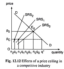
Also, at p_c < p₀, the demand for the good would be larger than the market equilibrium quantity, q₀, and the supply of the good would be smaller than q₀. Thus, a shortage of the good would develop in the short run. We may illustrate all these points and what would happen in the long run with the help of Fig. 12.12.

In Fig. 12.12, the demand curve for the good is DD and, initially, the short-run supply (SRS) curve of the industry is SRS₀. Therefore, the market equilibrium price of the good is obtained to be p₀ at the point of intersection E₀ of the DD and SRS₀ curves.

Let us assume that at p = p₀, the typical firm in the industry produces an output of q = q₀ and earns just the normal profit, i.e., p₀ = the minimum average cost of the firm. If the number of firms is n₀, then the industry output at p = P₀ would be n₀q₀.

Let us now suppose that this price, p₀, is considered to be too high and the government imposes a ceiling price of p_c (< p₀). The immediate effect of this would be an increase in the demand for the good from n₀q₀ to q* and the decrease in supply from n₀qo to n₀q₁ where q₁(q₀) is the output a typical firm would produce at p = p_c.

Thus, the imposition of the ceiling will create an excess demand in the market of the amount q* – n₀q₁.

On the other side of the picture, the firms would earn now less than normal profit or they would have economic losses, since p_c is less than p₀ = minimum average cost. Therefore, in the long run, firms would be leaving the industry.

As the number of firms diminishes the SRS curve of the industry would be the summation of the short-run marginal cost (SMC) curves of a smaller number of firms and so the SRS curve would shift to the left.

This would cause the excess demand gap to widen. For example, if the number of firms diminishes to n₁ and the SRS curve shifts from SRS₀ to SRS₁, the excess demand gap becomes q* – n₁q₁ which is larger than the earlier gap. It may be noted that the supply of the industry now would be n₁q₁ where n₁ is the number of firms and q₁ is the output of each firm at p = p_c.

If the imposition of price ceiling continues even though the firms are earning economic losses and the excess demand gap has widened, more firms would leave the industry and the excess demand gap would widen more. For example, let us suppose that the number of firms has reduced to n₂ and the SRS curve has shifted to the position of SRS₂.

Now the industry supply would reduce to n₂q₁ although demand would remain the same at q* (at p = p_c). Therefore, the excess demand gap now would be still larger. It would now be q* – n₂q₁, and it would be larger than the previous gap since n₂q₁ < n₁q₁.

If the policy of imposing the ceiling price continues and things proceed further in the way as we have described, then, ultimately, all the firms would leave the industry. This simple analysis points to two interesting features of price control programmes that we observe in the real world.

First, shortages appear as soon as the price ceiling is imposed and they appear to become larger the longer the control continues. Also, in the creation and widening of the excess demand gap, a big—if not bigger—role is played by the dwindling supply. In the case of essential goods, the role of increasing demand may not be that strong.

Second, the longer the controls are in effect, the more the firms would leave the industry and, consequently, more the SRS curve would shift leftward, and higher would be the market- clearing price and lower would be the market-clearing quantity of the good.

Price Controls in Monopoly:

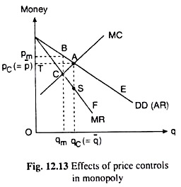
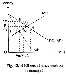
For the purpose of curbing the monopoly power, the monopolist may be brought under a system of price control, i.e., a price ceiling may be imposed upon his product. We may explain the effects of such price control with the help of Figs. 12.13 and 12.14.

In both these figures, the AR curve or the demand curve of the (pure) monopolist is the curve DD (AR) and his marginal revenue and marginal cost curves are, MR and MC respectively.

Also, in both these figures, the pure (unregulated) monopoly solution is (p_m, q_m), which is obtained at the point of intersection, C, of the MR and MC curves, and the competitive solution is (p_c, q_c), which is obtained at the point of intersection, A, between the DD curve and the MC curve.

This is because, if the monopolistic industry is converted into a competitive industry, the demand curve of the monopolist, DD, which is also the demand curve for the product would become the demand curve for the product of the competitive industry and the MC curve of the (multi-plant) monopolist would become the supply curve of the competitive industry or the supply curve of the product.

We shall see now that the effects of price control would depend upon whether the price ceiling, p_c, is equal to or lower or higher than the competitive price, p̅. In Fig. 12.13, we have assumed that p_c has been set equal to p̅. This implies that up to a demand of q_c (= q̅), p would be constant being equal to p_c (= p̅) , and thereafter as p falls, q rises. So, the demand curve would be TAE with a kink at the point A.

Consequently, the marginal revenue curve would have two parts, TA and SF, with a vertical discontinuity between these two parts, i.e., between the points A and S. This is because, for 0 < q ≤ q_c, the horizontal demand (AR) curve is also the MR curve and for q > q_c, the original MR curve is the marginal revenue curve.

Therefore, if the price ceiling is imposed at p_c (= p̅) , the monopolist’s MR = MC point would be the point A which is, of course, the competitive solution. Therefore, here the price control would compel the monopolist to take up the competitive solution (p̅, q̅) as his profit-maximising point.

As a result of the price control, p would be smaller than p_m and also q would be larger than q_m. Now there would be no loss of welfare due to monopoly, since the monopoly solution has become identical with the competitive solution. The loss of welfare of area ABC that was associated with the monopoly solution (p_m, q_m) would all be eliminated as p_c is set equal to p̅ and q̅ rises to q_c (= q̅).

It may be noted also that the price control will not develop here any excess demand problem, demand being equal to supply at p = p_c, both being equal to q_c.

Let us now refer to Fig. 12.14 and see what would be the effects of price ceiling if the ceiling price (p_c) is set lower than the competitive price (p̅), but above the pre-control MR = MC level, i.e., above the level of point C. If such a price ceiling is imposed, the monopolist’s DD (AR) curve would become TNE.

His MR curve, therefore, would be horizontal and coincide with his AR curve, up to the point N on the DD curve. Therefore, his MR = MC point now would be the point M and he would now sell an output of q_c at the price, p_c. As a result of price control, he would now sell a larger quantity q_c > q_m at a smaller price p_c < p_m.

The welfare loss due to monopoly would reduce from the area ABC to the area AB’M—the welfare loss would reduce, but it would not reduce to zero, since the monopolist is selling an output which is less than the competitive output (q_c < q̅). It may be noted here that at the solution (pc, qc), an excess demand or a shortage would develop in the market, since at p = p_c demand (TN) is greater than supply (TM).

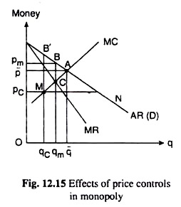
Let us note that the above results are obtained if the price ceiling p_c is set below the level of p but above the level of the point C. Now if p_c is set below the level of the point C, then the picture will be like that given in Fig. 12.15.

Here, after the price control is imposed, the MR = MC point is the point M where the monopolist would sell an output of q_c at the price p_c. This output is smaller than the pre-control monopoly output of q_m.

Besides, in this case, the loss of welfare due to monopoly will be more than what it was in the pre-control situation, since the output now is more less from the competitive output than from the monopoly output (q_m), (q̅ – q_c > q̅ – q_m).

The loss will increase from the area ABC to the area AB’M. Therefore, in this case, the market shortage would also be more than what it was in the previous case, since the point M will move from the right of the point C to its left. Therefore, the price ceiling will never be set below the level of the (pre-control) MR = MC at point C.

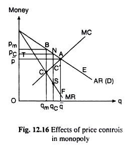
Lastly, let us see the effects of price control if the ceiling price, p_c, is set higher than the competitive price, p̅. We shall examine this case with the help of Fig. 12.16. After the imposition of the price ceiling, the AR curve of the monopolist would become TNE and his MR curve in two parts would be TN and SF.

The MC curve here has passed through the discontinuity between the two parts of the MR curve, i.e., in this case the MR = MC point does not exist. Therefore, here the monopolist would have to produce the output q_c and sell it at the price p_c.

At the N (p_c, q_c) point, his MR has not been equal to MC, rather MR = AR = p_c has been greater than MC. However, the monopolist would have to settle at this point for, if he increases his output even slightly, his MR along SF would be less than MC.

In this case, at the ceiling price p_c, the monopolist would sell the output q_c which is greater than q_m. That is, the imposition of the price control would be able to force the monopolist to sell a larger quantity.

Since q here is larger than q_m, but smaller than q, the welfare loss due to monopoly would exist but it would be smaller (= area ANC’) than what it would have been in the case of unregulated monopoly, the latter being equal to area ABC.

We should now mention one last point, i.e., there would be no market shortage in this case, since at p = p_c, the demand for the product would be equal to supply, both being equal to TN or q_c.

This case is similar to the case depicted in Fig. 12.15, where p_c < p, in all respects but two.

First, in the earlier case, a market shortage would develop after the price ceiling is imposed whereas in this case there would be no such shortage.

Second, in the earlier case, we have got p_c = MC at the post-control equilibrium point M(p_c, qc) and in this case, we have got p_c > MC at the post-control equilibrium point N(p_c, qc). That is why, in the post-control situation, profit would be smaller in the earlier case than what it would be in this case.